
UNBALANCED FACTORIAL DESIGNS The Long and The Short of It I suspect there are some people who won't want to read a tutorial this long--and it is the longest one by quite a bit--to find out how to deal with unbalanced factorial designs. It's not a simple issue, and there is no universally accepted answer. To quickly summarize, when a factorial design is balanced, the factors are independent of each other. "Orthogonal" is the word that is commonly used, meaning they are uncorrelated or unconfounded. In this case, any statistical software should give the "right" answer, as there is no dispute over how the calculations should be done. The problem arises in unbalanced designs because the factors are no longer orthogonal. Because the factors are confounded, they "explain" overlapping parts of the total variability, a problem most frequently encountered in multiple regression analyses where the explanatory variables are almost always correlated to some degree. The problem arises then in trying to figure out how to tease apart these confounds. How should the total variability be partitioned among the the various main effects and interactions? Three methods are in common use, some more commonly than others! There isn't even uniform agreement on what these methods should be called, so I'm going to adopt what has become known as the "SAS terminology." The issue is over how to calculate the sums of squares, and the SAS people refer to the three methods as Type I (or Type I sums of squares, but I will shorten it to Type I, Type I tests, or Type I analysis), Type II, and Type III. (Note: Not to be confused with Type I and Type II error, which is an entirely different thing. To keep them straight, in this tutorial I'll refer to the Type I error rate as the false positive rate.) Different statistical software packages use different methods by default. R uses Type I sums of squares by default, arguing quite vigorously in some instances that there are no other "types of sums of squares." (See this reference, for example.) Most of the large commercial packages, such as SAS, SPSS, and Minitab, use Type III (although the others are available as options). I will explain the differences below. I will try to explain what each of these methods does, because I think a well informed statistical analysis is a better statistical analysis. I will also try to justify the recommendations that I am about to give. But for this moment, to satisfy the people who just want to get an analysis on paper, let me tell you what I would do. (Which, of course, MUST be absolutely correct!:) Be forewarned. I can only give you a partial recommedation at this time. If the design is balanced, there is no issue. All three methods give the same result. I'm not sure those results are intended to be interpreted the same way, but they will give you the same numbers. It's when the design is unbalanced that you have to start to think about this. If the design is a true experimental design, by which I mean subjects have been randomly assigned to conditions within the experiment, and the design is mildly unbalanced for one of the following reasons:
If the design is unbalanced for some other reason, for example, if the design is quasi-experimental, using intact groups rather than random assignment to conditions, making it likely that the unbalanced condition reflects what is true in the population (the sample is unbalanced because the population is unbalanced), then the choice of an analysis is much more difficult. This is especially true if the design is more than mildly unbalanced, as I hope to demonstrate, or in the presence of an interaction that is unclear, i.e., marginally significant or not significant but still suspiciously large. In this case, you should choose an appropriate analysis depending upon what your hypotheses are and why the analysis is being done in the first place, i.e., what you hope to find out. In the nonexperimental case, if you must have something that resembles a traditional ANOVA, then Type II is the clear choice, but be sure you're aware of the problems with Type II tests when an interaction, significant or not, is in force. I know that's not very helpful at this point. Let me say, if the design is only very mildly unbalanced, then it probably doesn't matter a whole lot which method you choose. Try all three, and if you get similar results, flip a coin. DO NOT choose a method because you like the result it gives. That would be called "fishing for statistics." If the three methods give you different results, however, then you're going to have to understand a lot of what follows. Sorry! In any event, you should state in the written description of your analysis how the analysis was done, i.e., what type sums of squares were calculated! When Should We Use Type III and Why? If you're reading these tutorials, then you're probably already an "R person" or an "R wannabe" or at least someone who's curious about R. You may already have heard Bill Venables or some other R big dog paraphrased: "Type III sums of squares--just say no!" Given that I'm not a big dog and have already recommended Type III for mildly unbalanced experimental data, I think I need quickly to justify that before R people brand me a heretic and stop reading! After you hear my arguments, you're free to stop reading if you like. So before I even tell you what they are, here's why I (and a lot of other people) think you should use Type III tests for unbalanced experimental data. There is ONE case where Type III makes sense, in my opinion, and that is when the design is mildly unbalanced and the cell sizes are random and meaningless with respect to the treatments. This is most likely to happen in a designed experiment in which subjects have been randomly assigned to treatment conditions, and there has been minor and random subject attrition, or minor data loss for other, random, reasons. I'll offer four arguments to support this assertion. First, if cell sizes are random with respect to treatments, which is to say, there is no force of nature creating these cell sizes, making them effectively meaningless to the interpretation of the data, then a method of analysis should be used in which differential cell sizes do not figure into the hypotheses being tested. Of the three types, the only one that does this is Type III. Second, if cell sizes are random and meaningless with respect to treatments, then there is no reason to believe that cell sizes would be the same or similar in a replication of the experiment. Therefore, if cell sizes are part of the hypotheses being tested, as they are in Type I and Type II tests, this could make replication of experimental results more difficult. Third, it is generally true in experimental research that the researcher is seeking to test hypotheses about main effects of the form: Where mu1, etc., are cell-frequency-independent population means. If we are adhering to this tradition, in which "no effect" means equality of the population means, and those means are estimated, as is traditional, by unweighted marginal means in the sample, then we are left with little choice as to a method of analysis. The only one of the methods that will test for the equality of population means estimated from the sample as unweighted marginals is Type III. How do we know that the population means are best estimated by the unweighted marginals? Venables comes right out and calls this an entirely arbitrary hypothesis. Perhaps the population means are better estimated by the weighting scheme that is used in the Type I or Type II method. I would consider this to be a strong argument if the DV were being measured on intact groups (i.e., a quasi-experimental design), but in experimental research, let's face it, the population is a fiction. There is no population of people who have been given a list of thirty words to memorize, no population of rats that have been injected with LSD, and no population of agricultural plots growing alfalfa and fertilized with...whatever, at least not one that we are sampling from. What I want to know is, if I tell this group to do this, and that group to do that, will it make a difference in the number of words they can recall? In this case, "no difference" is defined as equal means, or means equal enough that we can't be confident that the differences are due to anything other than random error. And if I have a second, cross-classified IV, then I'm not interested in seeing how that variable changes the outcome of my "this-that" variable. At least I'm not until I'm looking at the interaction, and presumably I already have. If there's an interaction, then I wouldn't be looking at the main effects. Thus, when I do decide to look at the main effects, I want the influence of one variable on the other removed. I don't want to see the effect of B above and beyond the effect of A. I want to see the effect of B after any and all variability due to A has been removed. That includes variability created by the possibility that A may have an interaction with B, even though we didn't find it significant. In other words, when I'm dealing with experimental data, I want the entire confound of A with B removed from the main effects. 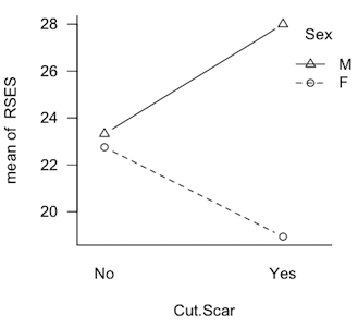
It's trickier than you might think. Take a look at the profile plot at left. These are plotted means from a quasi-experimental design that was seriously unbalanced. What effects do you see? Clearly there's an interaction, so perhaps we should stop there. But the interaction is not significant and, of course, if students were being asked to answer this question on a test, we'd also expect them to evaluate the main effects, and that's not so hard in this case. It looks like the "average Cut.Scar line" would be pretty much flat, so there is no main effect of Cut.Scar. The two "Sex lines" are clearly separated, however. The distance between the middle of those lines appears to be about 4-5 points. So a main effect of Sex is being shown. Is that how you did it? Is that how you teach your students to do it? Then you're evaluating the main effects using unweighted marginal means. You have effectively done a Type III analysis in your head. (And that would be the case even if there were no interaction, i.e., if the lines were parallel.) The Type II analysis finds just the reverse, a significant "main effect" of Cut.Scar (p=.02) and no significant "main effect" of Sex (p=.3). The interaction was not significant no matter what type sums of squares were calculated. (The Type III analysis finds p=.1 for the interaction, p=.9 for the main effect of Cut.Scar, and p=.06 for the main effect of Sex.) I hasten to point out that this is not a contrived data set. If the literature on unbalanced designs has taught us anything, it's that it is easy to contrive a set of data that make one or the other of the methods look bad. This is not one of those. These are real results from an actual study. They will be discussed in more detail below, where I will suggest using Type I tests to evaluate them. Fourth, yes, it's true that Type III tests on the main effects violate the principle of marginality (to be explained eventually), but such a violation is necessary in order that the tests have the above properties. As long as the unbalanced condition is mild, such a violation will have little effect on the outcome of the tests. Once again, in experimental research, I want to see the effect of B after A + A:B has been removed. If the design is balanced, and the effects are othogonal, then that is the same thing as saying effect of B after A is removed. If the design is not balanced, and the variables are not orthogonal, then to get the influence of A entirely removed, A:B also has to be removed. Yes, that's a violation of marginality, and to minimize any deleterious effects such a violation might cause, the design should be kept balanced, or as close to balanced as possible. "Yes, but if there is no interaction, why are we talking about A:B at all?" In experimental research, main effects are (almost) never interesting in the presence of an interaction, but interactions don't always show themselves. They don't always turn out to be statistically significant, that is. If we have every good reason to believe the interaction doesn't exist, then don't put it in the model to begin with. Don't analyze for it. Don't throw it out; don't even look for it. That's not usually the case, so the interaction ends up in the analysis, and it will have some of the total variability associated with it. That may be nothing but random error. Nevertheless, there it is, and it has to be dealt with. If the interaction is nonsignificant but still suspiciously large, then it might behoove the data analyst to find some other way to look at the "main effects" other than the traditional main effect tests. After all, traditional main effects are pretty much meaningless in the presence of an interaction, and just because it's not significant doesn't mean it isn't there. Hey, the Type III people play pretty rough with the Type II people on that issue, and here it is coming back to haunt you. Type III sums of squares DO NOT, by some miracle of mathematics, make it meaningful to look at main effects in the presence of an interaction! DO NOT take this as a blanket recommendation to use Type III tests in all cases. It most certainly is not. There are cases where Type III tests would be disasterously wrong. I hope to be able to point those out below. (Note: You can probably tell that I'm more a Fisherian than a Neyman-Pearson type when it comes to evaluating hypotheses. I'm not going to behave as if an effect isn't there just because the p-value didn't happen to slip below some magical criterion! I'm especially not going to do that when doing it might have a damaging impact on my interpretation of other effects!) Examples Before we get started, clear your workspace, and open a script window
(File > New Script in Windows; File > New Document on a Mac). Then very
carefully type (or copy and paste) the following lines into a script.
For these examples, we will look at a very simple, but unbalanced, two-way
factorial design. The data are in the MASS library.
When analyzing factorial data, we should always begin by checking for
balance. This can be done by crosstabulating the factors.
Type I Analysis This is easy because it's what R gives by default. Notice, however, that the
result is different depending upon the order in which the factors are entered into
the model formula. For this reason, most people do not like Type I, somewhat
unfairly in my opinion.
Type II Analysis The R base packages do not have a function for Type II tests. In this simple, two-factor case, it's not difficult to construct the Type II ANOVA summary table from what we've seen above. Notice that the interaction line and the residuals (error) line are the same in the two outputs. They will also be the same in a Type II analysis. It's the main effects that will be different. (Warning: These statements apply to the two-way design ONLY!) However, the second main effect in the tables above, Mother in the first table, and Litter in the second table, are essentially Type II tests. If you take the second line from each table, add the interaction and residual lines, you have a Type II ANOVA summary table. This will NOT be the case for more complex designs! For more complex designs, you should definitely resort to using the optional
"car" package, where Type II tests are the default. (The rationale for this is
explained by Fox and Weisberg, 2011, see Refs.)
Type III Analysis Buckle up! Here we go! There is also no built-in function for Type III tests,
and don't expect one anytime soon! To do Type III tests, you must be aware
of how you have your factor contrasts set. Treatment contrasts will NOT work.
WARNING! Here's something I learned the hard way. You may know that the aov() function does not have a problem with dichotomous IVs coded 0 and 1 when a Type I ANOVA is desired. R will figure it out. THIS IS NOT THE CASE with the aovIII() function. Make absolutely certain that any variable being fed to this function on the right side of the tilde is recognized as a factor. (Okay, still another note: The first line in the "car" output is a test that the intercept is zero, which is rarely of interest.)
Further Consideration of the "genotype" Data Notice in all the analyses we did above, the interaction term is always the same. The highest order effect term will always be the same no matter which of these analyses we choose. Thus, I guess one line of advice here might be "pray for an interaction." When the interaction term is significant, lower order effects are rarely of interest. What if the interaction term is not significant? In the two-way analysis, that means interest is focused on the main effects. But, should we drop the interaction term and redo the analysis without it before looking at main effects? Or should the interaction term be retained even though nonsignificant? Opinions differ. The majority consensus seems to be that nonsignificant interactions should be retained in the analysis. As I tell my students, nonsignificant does not mean nonexistent, and the existence of an interaction, significant or not, will eventually become an issue for us as we explore this topic. I'm not sure I agree with retaining the interaction. However, for now, I just want to point out one thing. If the interaction term(s) is (are) dropped, so that the model becomes additive (just main effects), Type II and Type III analyses will give the same result. Try it! We'll find out why below. Concerning Type I tests, if entering the factors in different orders gives different results, then those results surely have different interpretations. Correct! But we're not there yet. We'll get to interpretations below. If you just can't wait, there is an excellent discussion of this very problem in William Venables' Exegeses document. Be aware for now, however, that Type I tests are the ones that least resemble what most people think of as a traditional ANOVA.
A Special Case The "genotype" data did not present us with too very much of a problem, as the same effect, the "Mother main effect", was significant in all the analyses. That's a rather naive way to look at things, especially considering that the two "significant main effects of Mother" that we saw in the Type I analyses were not the same effect! But I'll let that slide for now. Suppose we have the following situation. If I remember, it was the mid 1970's when Hans Eysenck introduced what has come to be called the PEN model of human personality. PEN stands for psychoticism, extraversion, neuroticism, which are supposedly three major dimensions of personality, kind of like a 3D coordinate system within which everyone has a point determined by his or her scores on three scales. We're interested in his psychoticism scale, which supposedly measures, among possibly other things, a person's susceptiblity to developing a psychotic disorder such as schizophrenia. We might imagine that such susceptibility is a function of several variables. (I.e., you don't go crazy because of just one thing.) We're going to investigate two of those variables: genetic predisposition (do you have craziness among your immediate relatives, yes/no?); and childhood trauma (were you abused, bullied, deprived, a victim of loss, etc., as a child, yes/no?). Suppose we know the following facts from previous research. 1) 10% of people in the general population have a genetic predisposition, 90% do not. 2) 20% of people in the general population (of adults) experienced childhood trauma as we've defined it, 80% did not. 3) Experiencing childhood trauma does not make you any more or less likely to be genetically predisposed, and being genetically predisposed does not make you any more or less likely to experience childhood trauma. Thus, genetic predisposition and childhood trauma are independent of each other. (IMPORTANT NOTE: I'm not saying any of this is factual. I'm making this up for the sake of this example. I can easily image how fact 3, especially, could well be wrong!) Furthermore, suppose we also know the following. 1) In the general population, scores on the psychoticism scale have a possible range of 40-160, with a mean in the mid 90s and standard deviation of around 20. (I have NO IDEA if this is correct, but it doesn't matter for the sake of this example.) 2) The base level on the psychoticism scale for people with no predisposition and no trauma is, on the average, a score of 90 (ish). 2) The presence of childhood trauma adds 10 points to that. 3) The presence of a genetic predisposition adds 15 points to that. Here's what we don't know. What is the effect of having both trauma and predisposition? Is it additive? I.e., do the effects of the two factors simply add together to give the effect of both? In that case, the combined effect should be 25 points. Or do the two factors somehow interact with one another to make their combined effect greater than 25 points? Off to the grant writing workshop we go! Okay, we're funded, and we've taken a random sample of 100 people from the
general population. We've cross-classified them on the two factors of interest
to us, and we've come up with the following table. The numbers in the cells are
obtained sample sizes, n.
Since I made the cell frequencies come out perfectly, I might as well make the cell means and standard deviations come out perfectly as well. Here are the overall results.
All of the ANOVAs can be calculated from this information (in the 2x2 case
only; you'll learn how below). Here they are.
The tests lost quite a bit of power due to the unbalanced nature of the design. With a balanced design, if that had been possible, these main effects would have been found with as few as 16 subjects per cell (64 subjects total). Nevertheless, the Type I and Type II tests still found the main effects. We have to wonder why the Type III tests didn't find the main effects.
Wonder no longer. I'll show you. Notice this is the additive case in which
the interaction is exactly zero. Let's remove it from the model and see what
happens.
The following table shows the trauma main effect as it is being tested by each of the three types of tests (with the interaction included in the model, which is only relevant in the Type III case).
In each case, the sum of squares is calculated as the mean difference squared times the effective row size divided by 2. If the design were balanced, all three types would be testing the same effect. With proportional balance, Type I and Type II test the same effect, but Type III tests a different effect (same size mean difference but different means and difference in effective row size). When the interaction is deleted from the model, the main effects being tested by Type I and Type II don't change (although the error term will change a bit). However, when the interaction is deleted, the main effects being tested by Type III do change, and it's not easy to predict how they will change. This derives from the fact that in Type I and Type II tests the main effects and the interaction are orthogonal, while in Type III tests they are not (e.g., see Herr and Gaebelein, 1978). Thus, in Type III tests, if the interaction is deleted from the model, even if it is a zero interaction, the effects being tested as main effects will change somewhat unpredictably. I'll point out one more thing. Notice that the row marginal means being tested by Type I and Type II are the weighted means. This is typical for the first factor entered into a Type I test, but is not typical for Type II, where the weighting scheme is usually considerably stranger. Thus, when the design is proportionally balanced, Type I and Type II tests become the same, but that's not because Type I becomes Type II. It's because Type II becomes Type I. Those were additive main effects. The interaction was zero. It's interesting to see what happens when we add a weak and a strong interaction. Type I and Type II tests again give identical results, so only Type II and Type III are shown. The weak interaction on the left was created by adding 7 points to the mean of the lower right cell. The strong interaction on the right was created by adding 27 points (i.e., an additional 20 points). 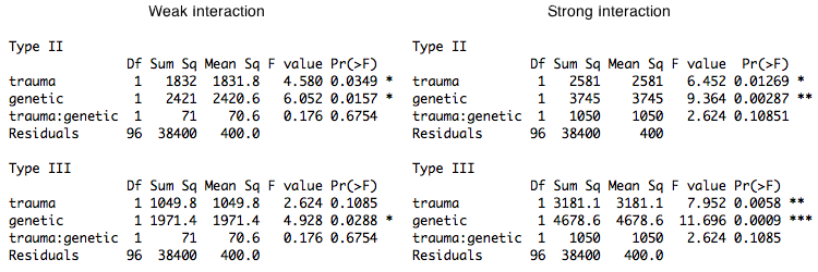
Let's look at the case of the weak interaction first. We have created this interaction by taking the largest of the four means
and making it even larger. Thus, in the ANOVA way of thinking, not only have we
created an interaction, but we have also increased the magnitude of the main
effects. (Think of the profile plot.) This is reflected in the increased size of
the sums of squares. Notice that the Type III sums of squares are still smaller
than they were above when there was no interaction and the main effects were
smaller. If we drop the tiny little interaction term from the model, as if by
magic all three analyses will give the same result.
In the case of the strong interaction, the interaction is now of the same
order of magnitude as the main effects, but still has not reached statistical
significance (because the unbalanced design lacks the power we need to see it).
What happens if we drop it?
These interactions were created by increasing the values of data points in a cell that had only 2 of the 100 subjects in the study, in a column that had only 10 of 100, and in a row that had only 20 of 100. These two data values determine 1 of our 4 cell means and, therefore, must be considered influential points. (Cook's D=.25 for both points, the highest values by far of any of the Cook's distances. Case 98, which is an outlier in the upper right cell has a Cook's D=.15.) The response of the Type III analysis to changing these values can politely be described as "exaggerated." (If I wanted to be somewhat less polite, I would use the word "goofy.") The Type III tests failed to find the main effects when the effects were additive and produced an exaggerated response to the creation of a nonadditive effect by changing the values of two highly influential points. I.e., the tests are not resistant to changes in influential values. This is because, as we'll see, the Type III tests weight all of the cell means equally. Thus, changing the values of two data points in a cell that has only 2, or in a column that has only 10, has a much greater influence on the analysis than changing the values of two data points in a cell that has 72 values would have. I'm going to commit an R heresey and say that it makes perfect sense (in my humble opinion) to weight the cell means equally when the cell frequencies are meaningless and the cell frequencies are not too different. This might happen in a randomized design with modest and random subject attrition. Weighting the cell means equally does not make sense when the cell frequencies are meaningful and disparate. Furthermore, changing the model from nonadditive to additive, which has no effect on the size of the main effects in the data, caused the Type III tests to change the evaluation of the main effects considerably, while the Type I and Type II tests changed hardly at all in their evaluation of the main effects. Notes Herr and Gaebelein (1978) suggest that dropping the interaction term in a
Type III analysis is not justified, because unlike in the Type I and Type II
case, the interaction sum of squares is not orthogonal to the main effects
sums of squares. "Because the sums of squares for rows and for columns are
orthogonal to the interaction sum of squares in EAD [N.B.-Type II], HRC, HCR
[N.B.-hierarchical rows then columns, hierarchical columns then rows, Type I],
and WTM [N.B.-weighted means analysis for both main effects], it would be
possible to pool the interaction sum of squares with error in these analyses
if it were felt that there was no interaction. This would not be possible in the
STP [N.B.-Type III] analysis, since the interaction sum of squares is not
orthogonal to either the sum of squares for rows or that for columns when the
cell sizes are unequal" (p. 212). For another take on the analysis of
proportional cell data, see Gocka (1973), as well as the various Overall and
Spiegel articles, responses to them, and responses to the responses.
Another Example: The Nature of the Problem In the previous section we saw an example of a "proportionally balanced" design, which was unbalanced, but which, nevertheless, had independent factors. (A chi square test on the cell frequencies would give a chi square of 0.) We saw that the Type III tests worked too hard at correcting a confound between the factors that really didn't exist. The following example shows what happens when the factors are clearly confounded. Many data sets, both real and artificial, have been offered up in various
textbooks and journal articles (e.g., the salary and gender bias data and the
psychotherapy for depression data in Maxwell & Delaney). The problem is perhaps
most straightforwardly illustrated by an artificial data set treated by Howell
and McConaughy (1982). These data, to which I have added a fourth variable to
be explained below, are shown here. (These data are not available in the data
sets file that accompanies these tutorials, so if you want them, copy and paste!)
Even a casual inspection of the data will illustrate the nature of the problem. Geriatric patients stay a lot longer (M = 20.9 days, SD = 1.02) than obstetric patients do (M = 2.9 days, SD = 0.83), and Hospital I cares mostly for obstetric patients (n = 10) and relatively few geriatric patients (n = 4), while for Hospital II it's just the reverse (n = 5 obstetric patients, n = 12 geriatric patients). Thus, "Hospital" is confounded with the kind of "Patient" being routinely seen, and straightforward calculation of mean Stay by Hospital presents a biased picture (M = 8.0 days, SD = 8.24 for Hospital I, versus M = 15.6 days, SD = 8.70 for Hospital II). Admittedly, these summary statistics are of questionable value due to the highly bimodal distribution of data within hospitals, but let's continue naively for a moment, performing a t-test to find that the difference in stay length is statisically significant, t(29) = 2.47, p = .02, two-tailed. The difference is quite large and "unmistakable" by the traditional Cohen's d criterion, d = 0.9. Clearly, Hospital II is being handed the unpleasant end of the stick in this analysis due to the relatively large percentage of geriatric patients cared for there. If we had no other information than what's in the variables Hospital and Stay, we'd be up a statistical creek at this point. A casual walk through the patient care wards of the two hospitals would surely tell us that we have a problem with confounding, but we'd have no data we could use in an attempt to remove this confound statistically. Fortunately, we have the Age variable, which we can use as a covariate. The
result of a regression analysis with both Age and Hospital entered as predictors
is shown next. The Age x Hospital interaction was nonsignificant, p = .6, so as
is often done in analysis of covariance (ANCOVA), it
has been removed from the analysis.
Suppose the Age variable was not available, as it was not in the original data
from Howell and McConaughy. Now we must rely on a 2x2 unbalanced factorial ANOVA
to get at the truth (and perhaps rightly so given the strongly bimodal nature of
the Age variable). We begin with an examination of the relevant means and group
sizes.
Before we proceed to the inferential tests, however, let me make a few relevant points about the design of this study. First, no subjects have been randomly assigned to any of the conditions of this study. It is an observational study, and both explanatory variables are quasi-independent variables. We might presume that the cell sizes are representative of the sizes of the sampled populations, although there is no guarantee of this and no way to tell from the data. In any event, the cell sizes are not different at random or by accident. Second, this is the simplest factorial design we can have, a 2x2 design with both variables being tested between groups. I.e., both variables will be tested on a single degree of freedom, which is not important in principle but turns out to be relevant in the calculations that follow. Third, we can see that we are unlikely to find a signficant interaction in these data, but, as I repeatedly try to hammer into my students, nonsignificant does not mean nonexistent! Perhaps more importantly, there seems (to me) to have been no way to predict a priori whether we should have expected to see an interaction or not. At long last, here are the results of the three different types of analyses.
It is relevant to the Type I tests only that Patient was entered first and
Hospital second.
Notice as this design is neither balanced nor proportionally balanced, the Type I and Type II tests (on the first factor entered) are now different. The Type II test is now much closer to Type III than it is to Type I. As we did in the previous section, it might be interesting to look at the actual Patient effect being tested by each type (Patient entered first and interaction in the model).
We see that all three tests show large sums of squares and substantial significance (if there is such a thing) in length of Stay by Patient type. Who's surprised? There is no significant effect of Hospital on Stay length, and the interaction is also not significant. In fact, all three types of analysis have yielded similar results. In this case, this is true ONLY because in the Type I tests we entered
Patient first and Hospital second. I would argue, given the hypothesis we are
interested in, that no one in his right mind would do those Type I tests the
other way around. But, rarely being accused of being in my right mind, I'm
going to do it anyway!
What The Heck Could It Possibly Mean? The Regression Solution. No! I am not going to show the least squares solution to unbalanced ANOVA. I'll refer you to any advanced textbook on ANOVA for that. Above, I mentioned that in multiple regression analysis it is par for the course to have correlated, and therefore confounded, predictors. How does regression analysis deal with that? I have this theory about gas mileage of cars. I think it's weight, and
weight only, that determines gas mileage. Once weight is controlled (held
constant, or however you want to say it), I don't
think horsepower or engine displacement matters a bit. I have some data
(admittedly from the 1970's) that I'm going to use to test this theory.
Wrong! We have not tested my theory as stated! In a standard regression analysis, each predictor is treated as if it is entered LAST into the regression analysis. In this analysis, we are looking at weight AFTER (or controlled for) horsepower and displacement, horsepower after weight and displacement, and displacement after weight and horsepower. That's usually what we want from a regression analysis, but not always, and not this time! I said "it's all weight." After weight is controlled, horsepower and displacement don't matter. That means look at weight first by itself, and we can see that it is the predictor that has the strongest correlation with mpg, r = -.868, although displacement is not far behind. Take weight out first, and THEN look at horsepower and displacement. That's a hierarchical regression. Without going to a whole lot of trouble, we can get something close to that
as follows.
Entering horsepower (hp) after weight increases R-squared by 83.274 / 1126.047 = 0.074, which doesn't seem like much, but it is significant, F = 11.96 on df = 1 and 28, p = .002. Entering displacement (disp) after weight and horsepower adds virtually nothing to R-squared. But hold on a minute! Why did horsepower get to go second? Why didn't
displacement get to go second?
Which should we believe? I didn't specify in my "theory" which should be
entered second and third. All I said was after weight, horsepower and
displacement add nothing. The only fair thing to do would be to add them in
together. In which case, R-squared would be increased by (31.639 + 51.692) /
1126.047 = 0.074. This would be tested on df = 2 and 28, so MS =
(31.639 + 51.692) / 2 = 41.6655, giving an F = 41.6655 / 6.964 = 5.983, and...
This is what the aov() function does. It does sequential or hierarchical tests. In the summary table, an effect is controlled for any effect that occurs ABOVE it in the table, but no effect that occurs BELOW it in the table. In ANOVA lingo, these are Type I tests. (A final note on cars: At least one of the interactions should be included in this model. I don't know which one. I didn't look. I left out the interactions to keep things simple.) The ANOVA Interpretation. In the cross-fostering study, we saw
these two ANOVA tables.
It's easier to decide in the case of the hospital analysis.
Which effect of Patient should we look at? Who cares?! We know what the
effect of Patient is! We're just including it as a control. I'm not even going
to look at it (unless I have to look at it as part of a significant
interaction). I do have an interesting question about Patient, however. If I
take out the effect of Age first, is there any variability in Stay length left
over for Patient to explain? Or is Patient merely a proxy for Age?
Now, tell me how we would get that information from Type II or Type III tests. Answer: We wouldn't! To summarize, the following Type I analysis... ... does these tests. Factor A is entered first and grabs all the variability it can get, uncontrolled for or ignoring B and the A:B interaction. Then factor B is entered and allowed a chance at whatever variability is left. That is, we are testing the effect of B after A, or removing A, or controlling for A, or holding A constant. We are not controlling either of these main effects for the interaction effect. Finally, the interaction is entered, and it is controlled for both A and B effects. Once again, in a Type I summary table, each effect is controlled for everything above it in the table and for nothing below it in the table. It is a series of sequential, nested tests. First A, then A + B, and finally A + B + A:B. We could do a similar thing as follows.
Type II Tests. Can't decide what order to put A and B in? Then do Type II tests. Type II tests treat all of the main effects equally, as if each main effect were the last one to be entered. Thus, all of the main effects are controlled for confounding with all of the other main effects, but the main effects are not controlled for the interaction effects. Type III Tests. Type III tests are the ones that most resemble a standard regression analysis, in that every effect is treated as if it were entered last. Everything in the table is controlled for confounding with everything else in the table. Thus, all of the main effects are treated equally in that all of the main effects are controlled for confounding with all of the other main effects, but in Type III, the main effects are also controlled for confounding with the interactions. I.e., the interactions are also taken out or removed before the main effects are tested. And therein lies a rather vigorous debate! Terminology Issues. If you go to the literature, you'll discover
that the SAS terminology is by no means universal, especially in older pubs
before the SAS terminology was developed. The following table shows some of
the other common names for these analyses, along with a summary in the last
column of what the tests do, where the vertical bar should be read as "given"
or "after" or "removing" or "controlling for".
How Do You "Control" For Something? Short answer: you hold it constant. Here is a summary of the hospital data
again, except this time I've given sums of squares in the cells instead of
standard deviations. (All of the values in this table are exact, i.e.,
unrounded.) At the bottom of the columns I've added two sets of means, the
weighted and the unweighted marginal means.
On the other hand, if we just blindly calculate (weighted) means at the bottom of the columns, we are ignoring the Patient factor, treating it as if it doesn't even exist, and then we end up in trouble with the confound. Patients in Hospital II stayed more than seven and a half days longer than patients in Hospital I, on average. Weighted means are weighted by the cell sizes, and that's what's causing the confounding here, the unequal cell sizes (unbalanced design). What if we calculate column means by weighting the cell means equally. Such means are called unweighted means. (Some people prefer to call them by the more logical name equally weighted means.) By doing this, we remove the effect of the unequal cell sizes and, thereby, remove the confound created by the unbalanced design. As you can see, the unweighted column means are almost identical. We calculated the unweighted means by making ALL the cell weights equal. Any value will give the same answer, so the easiest way would be to use 1, but just to make our lives interesting, let's use 6.315789. The column means are: Hospital I: (20.5 * 6.315789 + 3.0 * 6.315789) / (6.315789 + 6.315789) = 11.75Hospital II: (21.0 * 6.315789 + 2.6 * 6.315789) / (6.315789 + 6.315789) = 11.8 We would then use the same weights in calculating the unweighted row means. But to control Hospital for Patient, we don't have to make ALL the cell weights the same and, in fact, it may not be desirable to do so. Here's why. In the calculation of the interaction term in the 2x2 case, all four cell weights will be set to the same value, and this calculation will be done. Setting all the cell weights equal controls the interaction for the unbalanced condition in BOTH of the main effects, which is what we want. However, when calculating the main effects, setting ALL the cell weights equal not only controls one main effect for the unbalanced condition in the other, but it also controls the main effects for the unbalanced condition in the interaction. We may not want to do this. In the calculation of the Hospital main effect, to control Hospital for Patient, we do not need to set ALL the cell weights the same, they only need to be the same across each of the rows. That is, the weights for geriatric patients cells have to be the same, and the weights for obstetric patients cells have to be the same. Once again, as long as they are constant within rows, those weights can be anything, so let's make them 6 in the first row and 62/3 in the second row. ("I bet there's a reason you chose those particular values." You know me too well!) In this case, the balanced column means become: Hospital I: (20.5 * 6 + 3.0 * 62/3) / (6 + 62/3) = 11.28947Hospital II: (21.0 * 6 + 2.6 * 62/3) / (6 + 62/3) = 11.31579 Doing it this way controls Hospital for the unbalanced condition of Patient, but does not control Hospital for the unbalanced condition of the interaction. Now, let's find out why I chose those particular values. In a Type I analysis, if Hospital were entered first into a factorial
ANOVA, the sum of squares for Hospital would be calculated from the weighted
means, thus ignoring any possible confound with Patient. As we've seen, that's
not necessarily a bad thing, depending upon what you hope to find out from
your analysis. The calculation would be done this way: take the difference
between the weighted column means, square it, and multiply by the harmonic
mean of the column sizes divided by 2. (If this calculation sounds odd to you,
fiddle around algebraically with the t-test formula a bit. It's exactly what
you'd do in the course of calculating t2 between the two columns.)
In a Type III analysis, the sum of squares for Hospital would be
calculated from the unweighted column means. (Warning once again: ONLY in the
two-group or df=1 case!) Type III tests would control for the confound with
the second factor by calculating an effective sample size for the cells and
setting each cell size to that value. The effective cell size is just the
harmonic mean of the realized cell sizes.
You've no doubt noticed that the effective cell size is smaller than the arithmetic mean cell size, 7.75. This reflects the fact that an unbalanced design loses power to reject the null hypothesis compared to a balanced design. The more unbalanced the design is, the more power is lost. The Type II analysis is the most complex, but in the df=1 case, the logic is not hard to follow. For all the nashing of teeth that has occurred concerning Type II tests, they actually do something quite similar (or at least in the same vein) as Type III tests. They equalize the cell sizes where they need to be equalized to remove the confounding from a given factor. They just don't set ALL the cell sizes (or more appropriately, weights) to the same value. If we think of hypotheses as being about population values or parameters, then the point of calculating the marginal means is to estimate these population values. How best to do that? We've already seen two methods. One is to use the unweighted means of the cell means. I.e., we add up the cell means (in a row, for example) and divide by the number of them (the number of columns). Realized cell sizes are ignored (or used to calculate an effective cell size, which is actually quite irrelevant to calculating the unweighted means). Another method is called weighted means, in which the cell means are weighted by the cell sizes. This gives the mean of all the dependent variable values in a given row or column, as if the cross-classification were being ignored. We saw this when we examined the method called Type I. Thus, Type III, using unweighted means, statistically controls the confounding of the two factors created by the unequal realized cell sizes by setting all those cell sizes to an "effective cell size." Type I, using the weighted marginal means (for the first factor entered into the analysis only), does not attempt to control for the confounding, because it does not attempt to equalize the relevant cell sizes. Type III treats each cell mean equally but treats subjects differently. (Subjects in smaller cells count more that subjects in larger cells.) Type I treats each subject equally but treats the cell means differently. (Larger cells count more than smaller cells.) Type II also attempts to control the confounding but takes a somewhat different approach to estimating the marginal means. Consider the calculation of the mean square for error. It's based on the variances in each of the treatment cells, but it doesn't just add those variances and divide by the number of cells. Rather, a so-called pooled variance is calculated, in which the cell variances are weighted by the realized cell sizes. The idea is that estimates based on larger samples are likely to be more accurate, and so variances based on larger samples are weighted more heavily in the calculation of the estimated population variance (mean square error). The pooled variance will come out somewhat closer in value to the "more accurate" variances in the larger cells than to the "less accurate" variances in the smaller cells. The Type II tests do something similar in estimating the marginal means. The idea is that bigger (and more balanced) rows should have more impact on the column means than smaller (and less balanced) rows do. Once again, an "effective cell size" is calculated, but in the Type II
analysis it is calculated row by row rather than over the whole table (for the
column effect, that is). Once again, this is done by calculating harmonic means
of the realized cell sizes. In the calculation of a column effect (df=1 only!),
the "effective cell sizes" in the rows are set as follows.
For df>1 cases, a least squares regression method is used, and the above
calculations no longer work (except for error). But they convey the idea of
what the different analyses are attempting to do and how they either do or
don't attempt to control for confounds between the factors (and interacions)
due to unbalanced cell sizes. The following table summarizes this once again
for a somewhat more extreme 2x2 case than the one shown above, and perhaps
for that reason one that shows a little better what's happening. (We will
discuss these data below.)
For the record, in the regression method, which is equivalent to the above in
df=1 cases, but must be used in df>1 cases, the sum of squares is calculated by
comparing an enhanced model (i.e., a model containing the effect being evaluated)
with a reduced model (a model without that effect). The following table
summarizes this for the three Types of tests.
Type II tests especially have often been cast into the rubbish bin of statistical tests as testing "meaningless" (Howell & McConaughy, 1982) hypotheses about the marginal means. Indeed, when one looks at mathematical expressions of the hypotheses that are tested, one might be inclined to agree! You can find those expressions here, among other places. (Hint: If you're math phobic, don't click that link! You've been warned!) However, what it all boils down to after all the subscripts are accounted for is an attempt to control confounding by equalizing cell sizes where they need to be equalized, and in the case of Type II, NOT where they don't need to be equalized. I've Heard There's Some Sort of Issue With Interactions The differences among the three methods have to do with how they attempt to implement statistical control for the confounding that exists among the factors when the design is unbalanced. This is an issue only when it comes to testing the main effects (in a two-factor design). The interaction test (highest order interaction test) is the same in all three methods. So the issue with interactions is not that they test differently (at least not the highest order interaction). The issue is over how to interpret the main effects when an interaction is in force. First, when there is a nonzero interaction, should it be removed from the total variability before the main effects are evaluated? (Not removed as in deleted from the model but removed from the main effects.) In other words, should main effects be controlled for interactions? Should main effects ever be treated as if they were entered into the analysis after interactions? (Is Type III analysis ever justified?) The Type I/II people say, "No! Never! Such a stunt violates the principle of marginality." Marginality says that you should never include a higher-order term in your model unless all the lower order terms that are involved in it are also included. E.g., if we have AxB, then we must also have A and B. We can do DV ~ A + B + A:B, but we can't (or shouldn't) do DV ~ A + A:B. Yet this is exactly what Type III does when it controls main effects for interactions. In the course of running through the underlying math, models such as DV ~ A + A:B are used in the calculations. How seriously people take the principle of marginality seems to depend upon what type tests they have already decided to do. Type I/II people take it seriously. Type III people rarely mention it. It seems to me that the issue is a practical one. We all know that ANOVA is not a perfect technique that always yields the correct answer, and we all know it is sometimes used in imperfect circumstances. The issue should be, does violating (or not violating!) the principle of marginality damage the integrity of the calculations? The answer appears to be yes, in some circumstances it does (both ways!). So the question should not be, should we allow violations of the principle of marginality? It should be, when are those violations harmful, and when is failing to violate the principle harmful? The issue is dauntingly complex. A partial short answer would seem to be, if the imbalance in the design is mild or minor, it doesn't make much difference. If the imbalance is moderate or severe, it can make a huge difference. We are then faced with the question, which way is "correct?" Which way gives the "right answer?" The principle of marginality is more of a guide or a helpful suggestion than it is a law. When the design is more than mildly unbalanced, it can be a very good guide! Some people have argued that Type II tests (in particular) should never be used in the presence of a nonzero interaction, because they inflate the false positive rate for the main effects. This and testing "meaningless" hypotheses are probably the two stock criticisms of Type II tests. Other people have argued that in the presence of a nonzero but nonsignificant interaction, Type II tests should be used because they are more powerful at finding the main effects (Landsrud, 2003; Macnaughton, 1998). I find both of these argument dubious. First of all, if the interactions are dropped from the model, so that the model becomes additive, then Type II and Type III tests produce identical results. If the nonsignificant interactions are not dropped, then the correct statement is that Type II tests are usually more powerful. Sometimes that is not the case. At any rate, if the tests are more powerful because they are inflating the false positive rate for main effects, then choosing Type II tests based on the "more powerful" argument is dubious. (All of this assumes we are testing traditional main effects that appear in the marginal means.) The counter to the "more powerful" argument is that in the presence of a nonzero interaction, significant or not, Type II tests inflate the false positive rate. Based on Monte Carlo simulations I've done, testing for traditional main or marginal effects, this appears to be true, but only slightly. Based on the size of the inflation I've seen in simulations, I find this argument almost humorous when applied to a technique that is notorious for inflating false positive rates. In a two-factor design, we do three tests -- two main effects and one interaction -- EACH at an alpha of .05. In a three-factor design we do SEVEN tests, EACH at an alpha of .05. In higher order designs, the inflation problem only gets worse. To worry about inflating an alpha level from .05 to .055 by using Type II tests, the typical magnitude of inflation I observed in a 3x3 simulation, strikes me as being just a tad fussy. In 2x2 simulations, there was no inflation. I hasten to point out that these simulations were done with cases in which there were no marginal or interaction effects of any kind in the population but in which sampling error produced a nonzero interaction in the sample. Spector, Voissem, and Cone (1981) found false positive rates as high as .3 for the main effects in the presence of a significant interaction, using Overall and Spiegel's Method II (Type II analysis in the language of this article). In cases where there were no effects in the (simulated) population, the results of Spector and colleagues agreed closely with my results (minimal if any inflation). That's certainly a disturbing finding on the face of it. But I'm not surprised. This means that they were simulating cases in which the population contained an interaction but no main effects (otherwise the main effect would not be a false positive). This is the infamous "X-case" on the profile plot that gives students so much of a problem every semester in their research methods classes. It brings us face to face with the issue of whether it is meaningful to examine main effects in the presence of an interaction. Arguments have been made on both sides. Venables (1998) implied that it's "silly." Others (e.g., Howell & McConaughy, 1982) have suggested that it sometimes can be useful. 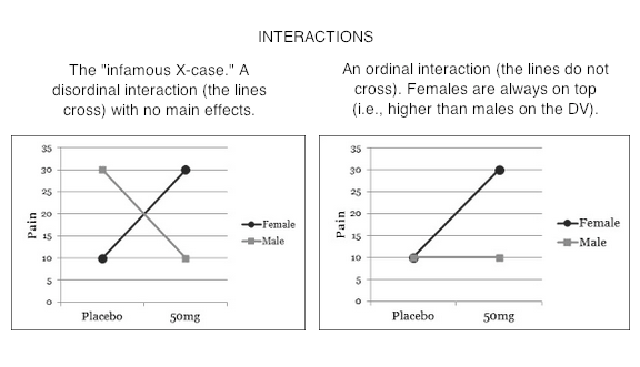
I ran simulations using this proportionally balanced design. Numbers in the
table represent cell frequencies or group sizes.
It is possible to have a two-factor interaction and only one marginal effect, in the case where the profile lines diverge. I simulated this condition in the current design by adding and subtracting respectively 1/2 sigma to the values at B3A1 and B3A3 and 1 sigma to the values at B4A1 and B4A3. In both Type II and III analyses, this interaction effect was found about 54-55% of the time. (Of course this result was the same for both types.) In the Type III analysis the A marginal effect was found about 50% of the time, and a false positive B marginal effect about 5% of the time. In the Type II analysis, the A marginal effect was found about 98% of the time, and a false positive B marginal effect was found 18-20% of the time. When the interaction was made to go in the opposite direction, i.e., the profile lines diverging more in the direction of the smaller groups (B1 and B2), the interaction was found about 40% of the time by both analyses. On the other hand, the Type III analysis was more successful at finding the A marginal effect than was Type II (52-54% of the time vs. 21% of the time). False positive rates for the B marginal effect remained inflated with the Type II analysis (12-14%) but were not inflated or only slightly inflated with the Type III analysis. But I tricked myself, didn't I? (As have some similar results published in reputable journals tricked me!) By making the lines diverge, I didn't create an ordinal interaction in the data, I created another disordinal interaction. Consider the following profile plots, which are from a study that we'll discuss in some detail below. 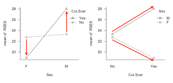
So once again, the inflation I was seeing in the previous simulation study may be a moot point. If we're seeing a disordinal interaction, we shouldn't even be looking at main effects. So yes, in the presence of a disordinal interaction, false positive rates for marginal effects that shouldn't exist can be substantially inflated in the Type II tests. What about when the interaction is ordinal? Here's the catch. You can't create an ordinal interaction in the above design without creating two marginal effects! You can't have false positives for marginal/main effects in such cases. Nevertheless, I ran simulations after creating an interaction as follows. In the above design, the A3 profile line was left flat. The A2 profile line was increased by 1/8 sigma at B1, 1/4 sigma at B2, 1/2 sigma at B3, and 3/4 sigma at B4. The A1 profile line was increased by twice those values. The Type II tests found the A marginal effect 93-95% of the time and the B marginal effect 17-18% of the time. The Type III tests did not do as well with the A effect (55-61%) but did better with the B effect (32-35%). Both types found the interaction 17-19% of the time. Then I reversed the direction of the interaction, placing the smaller effects at B4 and the larger effects at B1. The Type II tests found the A marginal effect 37-42% of the time and the B marginal effect 14-18% of the time. The Type III tests did better with both effects, finding the A effect 56-60% of the time and the B effect 25-29% of the time. The interaction was found 15-17% of the time. This still leaves us to cope with the disturbing case, as in the graphs above, of a disordinal interaction that is not statistically significant. Maybe we should just redouble our efforts to keep all our designs balanced? We can't! If we're taking a random sample from a population of intact groups, we take what we get! And if we don't, if we try subsequently to adjust those group sizes towards balance, so much for our random sample!
More on Interactions Those pesky interactions aren't done with us yet! I want to talk about two issues. 1) When is an interaction not an interaction, and vice versa? 2) Are main effects ever meaningful in the presence of an interaction? I found it necessary to temper my views on looking at main effects when there is an interaction in force because I'm a psychologist. In my own subfield, physiological psychology, we're stricter about measurement than most psychologists are, but even we do some stuff that hard science would consider pretty soft. When I was doing my dissertation research, I found it necessary to assess the emotionality of rats. I had several measures, but one was to pick the rat up and count the number of times I was bitten. (I was wearing a chain mail glove. Even grad school isn't that cruel!) You can almost expect one bite from a rat that hasn't been gentled. One bite doesn't mean much. But if the rat continues to gnaw on you, that is one POed rat! I seriously doubt that it is an interval scale of emotionality. If we're doing an experiment in which we give a subject a list of 30 words, and then some time later ask him or her to recall as many of the words as s/he can, we're not really interested in how many words a person can recall from a list of 30. How often does that come up?! We're interested in how some treatment we've applied has affected the subject's ability to memorize or recall. I doubt number of words recalled is a linear measure of that. Getting the first 6 or 7 is pretty easy. Then it gets harder, and by the time the subject has made it into the upper teens or lower twenties, each additional word recalled is a much more difficult chore. So does this graph show an interaction? 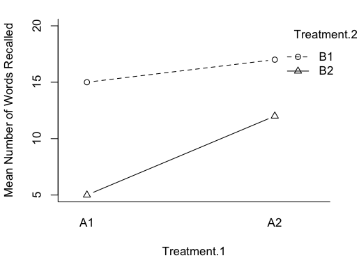
Or does it show an artifact of our scale of measurement? And if that's the case, then at least we have an interesting main effect or two to look at. Ramsey and Schafer, in their very excellent stat book, The Statistical Sleuth, discuss an experiment by Roger Fouts (1973) on American Sign Language learning by chimpanzees. Four chimps were taught the same 10 signs each, and interest was in differences among the chimps, and differences in difficulty of learning among the signs. The measure of how hard the sign was to learn was minutes to a criterion demonstrating that the sign had been mastered. It's a treatment-by-subjects design, a two-way classification without replication. As such, any variability due to what appears to be an interaction becomes the error term. There was an apparent chimp-by-sign interaction, and Ramsey and Schafer suggested making it go away with a log transform of the DV. What if that interaction was real and not just noise? It was obvious on the minutes scale, but not apparent on the log(minutes) scale. Which is the "real" measure of sign learning difficulty? In some of the "softer" areas of psychology, measurements are frequently on rating scales. "How much do you like chocolate? 1 means yuck, and 7 means totally addicted." What do the values on that scale mean? In the soft sciences, we have issues with measurement scales, ceiling effects, floor effects, etc. So when is an interaction REALLY an interaction? And if it looks like one but really isn't, should we then be looking at the main effects? If the measurement is a "hard" measurement, then those issues go away. If the measurement is a "hard" measurement, should we ever look at main effects in the presence of an interaction? Never say never, so I'll say almost never. There might be some practical value. It could help me make a decision as to which product I should stock in my store, even though the profitability of the candidates is not equally different over months or seasons. But in a scientific setting, if we're attempting to answer questions about what nature is like, and it's a "hard" interaction, then no. If there is an interaction, THAT is THE effect of interest. Recall the issue we had with the hospital problem when we used the age of the patients as a covariate. The mean age of the patients was 50.2 years, so we used that value to calculate adjusted mean stay length for obstetric and geriatric patients, even though there were no patients in our sample with an age anywhere near that. Was it an unjustified extrapolation? When the explanatory variable is not numeric but a factor, the issue becomes almost comical. 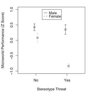
An interesting discussion occurred at myowelt.blogspot.com concerning an experiment that produced the graph at right. The design was unbalanced, and the researcher wanted to know how to get the same ANOVA result in R as he was getting in SPSS. Having looked into it, he ran smack into this issue of whether main effects should ever be entered into an ANOVA after an interaction, and if there is an interaction (as there is here), do the main effects even make sense. I particularly enjoyed the comment of Ista Zahn. "With respect to the specific analysis you describe here: As I understand it, it really doesn't make sense to talk about main effects for either gender or stereotype threat. The gender main effect here refers to the effect of gender averaged across levels of stereotype threat. In other words, it is telling you the effect of gender at a non-observed value of stereotype threat that is halfway between Yes and No. Likewise, the stereotype threat main effect is giving you the effect of stereotype threat at a value halfway between male and female, which makes even less sense. What I think you want to do is test the effect of stereotype threat separately at male and female, and to test the effect of male vs. female at high and low stereotype threat." How much better could that be explained? When you have an interaction, you do not look at main effects, you look at simple effects. I.e., you look at the effect of one variable at each level separately of the other variable. If we have an interaction, we don't need to worry about whether there is inflation in the false positive rate for main effects, because we're not going to be looking at main effects. The problem is not solved, however. There is still the issue of nonsignificant interactions. As I tell my students, nonsignificant does not mean nonexistent. A nonsignificant interaction could, in fact, be a very real interaction. If it's nonsignificant, should we just behave as if it doesn't exist? And how nonsignificant does it have to be before we can do that? This gets into issues of null hypothesis significance testing, and whether there is a meaningful difference between p = .045 and p = .055, and I'm just not going to go there!
Lessons From A Higher-Order Design If you think it's bad enough already, then you're really going to find this
unpleasant! Restricting our discussion to the simplest possible case of a two-way
design makes things seem simpler than they really are! Aitkin (1978) discussed
the analysis of a four-way design, and thanks to the good people at the
R-Project, we have those data.
I don't know what SPSS* or SAS would do with these data, but
neither aovIII() nor
Anova( , type=3) from the "car" package will produce a meaningful result.
I suspect this is due to the empty cells in the design. (*See the
footnote at the end of this section for an update on that statement about SPSS.)
First, let's look at the 4-way interaction. Why is it evaluated on df=2 and not df=1*1*3*1=3? Once again, that has to do with the empty cells. Notice that it's not significant. (The aovIII function returned this same result.) Second, let's look at the Lrn main effect. In the Type I table, Lrn is entered after Eth, Sex, and Age, and therefore is controlled for possible confounds with all the other factors. The SS = 689.288. What's happening in the Type II table? Why isn't it the same? Aren't Type II main effects controlled for possible confounds with all the other main effects? Yes, but Type II main effects are also controlled for all of the higher order effects that don't include them. Lrn, for example, is not only entered after Eth, Sex, and Age, but also after Eth:Sex, Eth:Age, Sex:Age, and Eth:Sex:Age. In other words, the Type II analysis is very thorough at removing the effects of other variables before evaluating a main effect, and that includes effects of other variables that might be part of an interaction not involving the variable under consideration. In evaluating the Lrn main effect, for example, the Type II analysis removes all variability due to Eth*Sex*Age first. Third, same comment for the interactions. From our discussion of the two-way design, we might be led to expect that the last two-way interaction, Age:Lrn, should come out the same in a Type I vs. Type II analysis. Nope again, and this time I'm not entirely sure why! But something is clearly removed (or not removed!) in the Type II analysis that is not (is!) in the Type I analysis. If you really need to know, I suggest you consult Fox and Weisberg (2011), because if they don't explain it, probably nobody will! (Note: At the website of the University of North Texas, Research and Statistical Support, I found the following statement. "Type II - Calculates the sum of squares of an effect in the model adjusted for all other 'appropriate' effects where an appropriate effect is an effect that does not contain the effect being examined." Does that mean Age:Lrn is also adjusted for Eth:Sex:Age and Eth:Sex:Lrn? I don't know, but that appears to be the case.) Fortunately for me, for the analysis that I am going to suggest, I don't need to know! But before we get to that, I suspect a lot of people would do here whatever their statistical software allows them to do and would give it no further thought. Bad idea! What's the point of doing a statistical analysis that you don't understand? For example, SAS allows an analysis using what are called Type IV sums of squares, which are intended for cases in which there are empty cells in the design. When there are no empty cells, Type IV defaults to Type III. I would bet my paycheck that a lot of SAS users would just run these data through SAS and take whatever they're given without really understanding what it is. These people should be banned from using statistical software altogether! I'll say the same for people who use SPSS and just take whatever SPSS spits at them without knowing the first thing about what "Type III sums of squares" really means. After all, it's SPSS. How can it be wrong? At one time, I confess, that would have included me! My stat professor from grad school used to say, if you are running a high-order ANOVA, pray you don't get a high-order interaction, because then you have to explain it! I know some people who don't even look at interactions higher than third order, because who can understand them anyway? I don't know about the soundness of that logic. I'll just say, phew! We don't have a 4-way interaction here! Where do we go next? I'm going to say, delete the 4-way interaction from the model, and
start looking at the 3-ways. I would do that as follows (following Venables
and Ripley).
Instead of guiding our model selection using p-values, we could instead be using AIC values. AIC means Akaike Information Criterion. Look at the Type II tests again on the 2-ways, except this time look at the column labeled AIC. The table shows the effect of deleting the 2-way interactions one at a time. Any deletion that decreases the AIC value is a deletion that should be done, according to this criterion. Thus, the p-value criterion and the AIC are telling us to delete the same four 2-way interactions. Nice! However, take a look back at the 3-way interactions. If we were using AIC as our model selection criterion, two of those would have been retained. AIC is not terribly well known in the social sciences, at least not yet, but there are some compelling arguments for using it as a model selection criterion instead of p-values. Something you might watch out for as we social scientists become more sophisticated in our model building. I'll have reason to mention it again in a later section. Okay, let's fillet the model.
If at this point an ignorant journal editor says, "No. I want Type III
sums of squares," here they are.
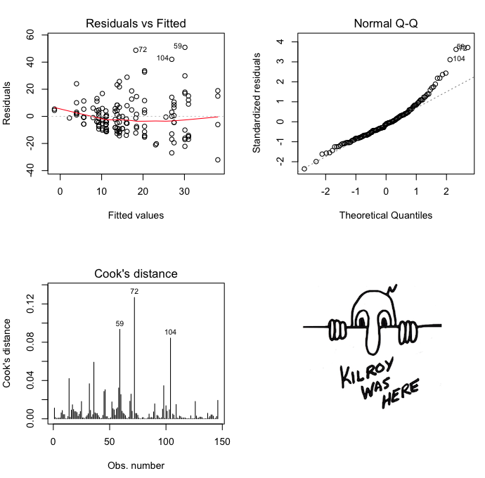
Here are some diagnostics on the model, suggesting
considerable heteroscedasticity. Venables and Ripley's log transform might be
a good idea.
> par(mfrow=c(1,2)) > with(quine,interaction.plot(Age,Sex,Days,type="b",pch=1:2,bty="l")) > with(quine,interaction.plot(Age,Eth,Days,type="b",pch=1:2,bty="l")) 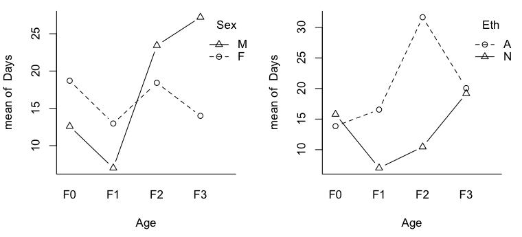
Now we can see why talking about main effects in the presence of interactions is inappropriate. It would certainly be an injustice to the Aboriginal kids in F0 and F3 to make a global statement of the sort, "Aboriginal kids miss more days of school, on average, than non-Aboriginal kids." It would also be misleading, even though there is no main effect of Sex, to say, "There is no difference, on average, in attendance by boys vs. girls." This may not be true in any of the age groups. Out of curiosity, I also plotted the nonsignificant 2-way interactions. 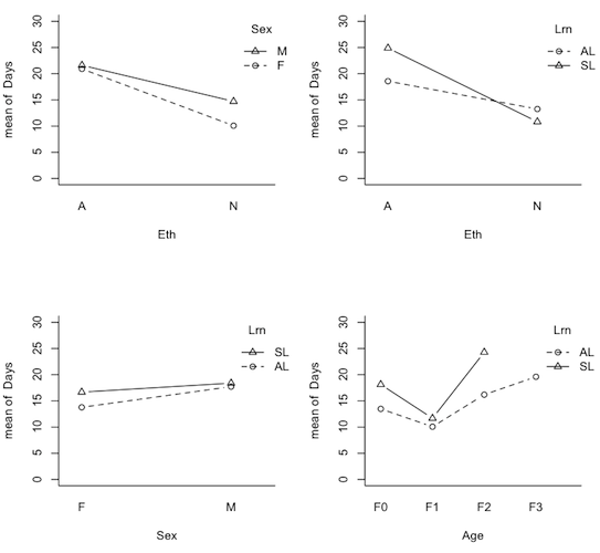
Note: Milligan et al, 1987, assessed the robustness of all three methods of analysis (i.e., all "Types") to heterogeneity of variance when the design is unbalanced and found all three to be not at all robust. The worst patterns were when cell variances were correlated with cell sizes. "The user is cautioned against collecting such data." This is not a problem unique to unbalanced factorial designs, however. It has been well known in the case of unbalanced single-factor designs for some time. Which doesn't mitigate its seriousness. A final note: Notice that the model we ended up with, with the four main effects and two interactions, is pretty close to what the Type II tests gave us right from the get-go. So why did I put myself through so much rigmarole? Because I understand this analysis. I do not understand an ANOVA table that has eleven interactions in it. Also, in the original analysis, I was doing 15 tests all at an alpha of .05. Now I'm doing 6, and all but one are significant. Familywise error can take a hike!
Some Notes on the Justifications for Deleting Interactions First of all, perhaps I should say that "deleting interactions" is a misstatement. They're not actually being deleted, they're being pooled with the error term. The literature on pooling interactions with the error term is almost as confusing as the literature on unbalanced designs! The primary argument against pooling/deleting (I'll say deleting) is, how do you know when to do it? The following arguments have been made. (Note: That I am aware of. I'm not going to plow through my stack of photocopied journal articles--yes, I'm old school--to find the appropriate references, but these points should NOT be credited to me!) 1) A significance test that fails to produce p<.05 is not an adequate reason for rejecting the existence of an interaction. (In your face, Neyman and Pearson!) 2) If you have every reason to believe that an interaction is unimportant, then it shouldn't have been included in the model to begin with. 3) Deleting interaction terms (i.e., pooling their variability with error variability) reduces the power of the tests for main effects. 4) In ten-way or fourteen-way ANOVAs, a few significant interactions can get lost in a sea of nonsignificant ones. 5) Deleting an interaction makes the implicit assumption that its magnitude in the population is zero. This is unlikely to be true. 6) You may have failed to find an interaction that actually exists because your test lacks power. 7) Deleting interactions in Type III tests produces an incorrect error term for testing main effects. To which I would reply: 1) Correct. As I've said repeatedly in this article, nonsignificant does not mean nonexistent. 2) Not including it automatically pools it with the error term in any kind of ANOVA that I'm aware of. 3) If you've decided, for either practical reasons or for theoretical ones, that an interaction "doesn't exist," then the variability associated with it, in your opinion, is to be treated as random error, and random error BELONGS in the error term. You're not reducing your power by pooling those terms, you're artificially inflating your power by not pooling them. On the other hand, if you're not really certain, but you have an interaction that you've just decided "not to make a fuss over," then that's a harder case. Not deleting "just in case" will (perhaps artificially) maximize the power of your main effects tests, while deleting will produce a conservative test. 4) Seriously? Who does this? 5) Well, yeah. But let's face it, statistics is a messy business. We make all kinds of assumptions that are false, like homogeneity of variance, for example. How likely is it that homogeneity is exactly true? It doesn't need to be, it just needs to be close enough. I don't claim to be perfect. I'm just trying to figure out how to do the best I can, and if I think deleting an interaction will help me do that, then that interaction is gone! The cardinal sin here would be failing to inform my readers of what I've done and why. If I'm truthful about what terms I've dropped and why, then they can decide for themselves if what I've done is justified. 6) Whose fault is that? 7) Gasp! These very same people have sometimes then turned right around and argued that nonsignificant interactions in Type II tests MUST be deleted in order to provide the correct error term for main effects tests. As we've seen, deleting the interactions in Type III and Type II tests produces exactly the same main effects tests. Since I'm reserving Type III tests for mildly unbalanced experimental data (and this is one reason why!), I'll just say, don't delete your interactions in those cases! The only one of these arguments that I'll take seriously is the first one. As I've already said, just because a significance test fails to produce a p-value that slips below some magical criterion, that's not a good reason for deciding that something doesn't exist. Statistical analysis is an intellectual exercise. Although it can be done without thinking, especially in these days of high powered statistical software, it certainly shouldn't be. Here are my arguments in favor of deleting interactions that you've decided, for one reason or another, are unimportant.
An Educational Example of Nonexperimental Data (Important preliminary note: As quasi-experimental designs go, this one is not very complex. It is quasi-experimental only in that it does not make use of random assignment to treatment conditions. Since the study looked at intact groups without any further attempt at control, some people might find it more reasonable to call this an observational study.) A few years ago (Spring 2013), Zach Rizutto, a student in our department, did a very interesting senior research project. Zach administered a survey to CCU students, which collected information on several factors about them. He also administered the Rosenberg Self-Esteem Scale. Most of the questions were included to cleverly disguise his real interest, which was to see if there is a relationhship between body cutting and scarification and self-esteem. He collected information on these variables:
> summary(scar)
 Sex    Cut.Scar       RSES
 F:80   No :124   Min.   : 7.00
 M:60   Yes: 16   1st Qu.:19.00
                  Median :23.00
                  Mean   :22.62
                  3rd Qu.:27.00
                  Max.   :30.00

> with(scar, tapply(RSES, list(Cut.Scar, Sex), mean))
           F        M
No  22.75385 23.32203
Yes 18.93333 28.00000

> with(scar, tapply(RSES, list(Cut.Scar, Sex), var))
           F        M
No  21.81346 25.18761
Yes 24.78095       NA

> with(scar, tapply(RSES, list(Cut.Scar, Sex), length))
     F  M
No  65 59
Yes 15  1

> with(scar, tapply(RSES, Sex, mean))            # weighted means Sex
      F       M
22.0375 23.4000

> with(scar, tapply(RSES, Cut.Scar, mean))       # weighted means Cut.Scar
      No      Yes
23.02419 19.50000

> with(scar, tapply(RSES, list(Cut.Scar,Sex), mean)) -> means
> colMeans(means)                                # unweighted means Sex
       F        M
20.84359 25.66102
> rowMeans(means)                                # unweighted means Cut.Scar
      No      Yes
23.03794 23.46667
You've seen the interaction plot already, but just as a reminder, here it is
again. Zach collected information from 140 students, not a bad sample size
considering he had only one semester to complete the study. Out of 140
subjects, he found one male cutter. The whole analysis hinges on how
representative that one score is. For the moment, let's assume that our one
sampled male cutter represents the population of male cutters.
Thus, we can see from looking at the interaction (profile) plot that we have an interaction between Sex and Cut.Scar. We see that there is not much difference in the self-esteem of male and female noncutters, t(122) = 0.653, p = .515, two-tailed. There appears to be a much larger difference in the self-esteem of male and female cutters. Male cutters have higher self-esteem than male noncutters, but female cutters have lower self-esteem than female noncutters. Hence, these simple effects go in opposite directions, and this qualifies as a disordinal interaction, as discussed previously. However, due to the small sample size of cutters, and the unbalanced nature of the data, the Sex difference at this level of Cut.Scar is also not statistically significant, t(14) = 1.76, p = .0996, two-tailed. The difference of over 9 points is about two standard deviations, so the effect size is very large, and if this condition had been more closely balanced, this would have been a highly significant difference, p = .004. But the population isn't like that, or so we are led to believe from this sample. There appear to be many more female cutters than male cutters, chi-sq = 8.27, df = 1, p = .004, with a Yates correction for continuity. Here are the Type I and Type III ANOVA summary tables.
First, let me address the interaction for a minute. I said above that a design loses power the more unbalanced it becomes. Had the cutters been more equally balanced between males and females, would we be looking at a significant interaction here? Maxwell and Delaney (see Refs) show that a 2x2 interaction in a nonorthogonal design can be calculated as follows. > harm.mean=function(x) 1/mean(1/x) # I keep erasing it! > harm.mean(c(65,59,15,1)) * (22.75385 - 18.93333 - 23.32203 + 28.00000)^2 / 4 [1] 65.7182If the design had been more balanced with respect to cutters (and assuming homogeneity of variance is preserved), the interaction would test like this. > harm.mean(c(65,59,8,7)) * (22.75385 - 18.93333 - 23.32203 + 28.00000)^2 / 4 [1] 240.5947 > 240.5947 / 23.56 # get an F [1] 10.212 > pf(10.212, 1, 136, lower=F) # get the p-value [1] 0.001734847In fact, if we'd had 14 female cutters and 2 male cutters, preserving the means and homogeneity of variance, the SSAB = 119.6238, and F(1,136) = 5.08, p = .03. We are paying a heavy price for having such an unbalanced design, but if this is what nature looks like, then it is a price we have no choice but to pay. (All of this assumes, of course, that our one male cutter is representative of male cutters. It is NOT, however, making a statistical error with respect to the error term. If I turned some of my female cutters into male cutters, the sum of squares would go down in the Female-Y cell and up in the Male-Y cell. Assuming homogeneity is preserved, the sum of these within cell SSes would remain close to the same.) I remember suggesting a drop1() on the
Type I analysis. I still have the result of that in my notes. (Apparently, I
don't throw anything away but the data!!)
If we drop the interaction, then both the Type II and Type III tests come
out like this.
First of all, the Type I tests with Sex entered first (because we wanted to see the effect of Cut.Scar with Sex removed) are telling us there is no significant effect of Sex because there isn't. Sex by itself, ignoring everything else, is not a significant predictor of RSES, t(138) = 1.61, p = .11, two-tailed. This is very similar to the ANOVA result. As we've seen, it's also not significant at either level of gender considered alone. The effect means being tested by the Type I test, as well as by the t-test, are 22.0375 and 23.4000. Not much difference there. Is that interesting? Heck yeah, that's interesting! I thought the women would come out a little lower, because they usually do. But they didn't. Good for them! Maybe things are changing here at the good ol' U of CC. Second, the Type I tests with Cut.Scar entered first are telling us there is a significant effect of Cut.Scar (ignoring Sex) because there is, t(138) = 2.72, p = .007, two-tailed, testing the means 23.02419 and 19.50000. Overall, cutters have lower self-esteem than noncutters. Fewer of those cutters are men, but who was asking? "But what if there were more male cutters?" Well, there aren't! That's the Type III question. What if there were the same number of male cutters as female cutters, and the same number of cutters as noncutters? That would be a very sensible question to ask if these were experimental data with randomly assigned subjects. But they're not. Provided the sampling was done adequately, these cell sizes represent something that's true in nature. There are many more female cutters than male cutters, and many more noncutters than cutters. "Oh, I see! If I want to see the 'pure effect' of a variable, I look at the first line, and if I want to see the effect of one thing controlled for the other, I look at the second line. I get it now!" Well, just hold up a minute. It's not that simple. The second line of the Type I tests are, in effect, the Type II tests. Supposedly, the Type II tests on the main effects do control one variable for the other, i.e., the second lines of the Type I tests are "B given A," "B controlled for A," "B after A is removed," etc. But the Type III tests also claim to control B for A, and as we can see, there is a huge difference in what we're being told by the two tests. I'm going to defer at length to John Fox. Dr. Fox is the creator and
maintainer of the "car" package and a major advocate of Type II tests. The
following was posted at the
R-help mailing list.
I cited the whole thing because it's an excellent summary of this controversy, but I call particular attention to one statement: "If, however, interactions are present, then the type-II tests for A and B are not tests of main effects in a reasonable interpretation of that term." In other words, Type II tests for main effects DON'T WORK in the presence of interactions. This same point was made in a somewhat less clear-headed way in the last section of this article. Since we have decided that the interaction is important (I've decided that), we shouldn't be looking at main effects in the Type II tests. We shouldn't be looking at them in the Type III tests either, but at least the claim has been made (in other sources) that the Type III tests test them "correctly" in the presence of an interaction. "So are the Type III tests correct here after all?" Nope! "Should we have pooled the interaction with the error term if we want to look at the main effects?" Certainly not! An interaction that is considered important should never be dumped into the error term! Two points. (I'm getting behind in my "points" here!) First, I disagree with Dr. Fox that the test on A (first factor entered) in the Type I tests "does not test the A main effect in any reasonable interpretation of that term." Sure it does! And I hope I've already demonstrated that. The A effect does not have to be "the partial relationship between the response and A conditional on B." A ignoring B is a perfectly reasonable definition of an effect. It all depends on what you're interested in looking for, i.e., what your hypotheses are. (Okay, let's not get tangled in terminology here. If you want to reserve the term "main effect" for "A conditional on B," fine! But A ignoring B is a perfectly reasonable definition of an EFFECT of A, and it's one that might very well be interesting.) Second, the question of whether or not Type III tests test main effects "correctly" in the presence of an interaction once again depends upon what you think a main effect is. If by "main effect" you mean an effect that answers the question, "What if there were the same number of male cutters as female cutters, and the same number of cutters as noncutters?" then sure, Type III tests are reasonable. But is that a reasonable question? Nature just isn't like that. Why would anyone want to pretend it is? Let me point out, it's not our analysis that is creating the confound between Sex and Cut.Scar. These effects are confounded in nature! Artificially removing the confound by some statistical trick seems to me to be doing a disservice to the phenomenon we are investigating, all in the interest of making our statistical analysis "easier to interpret." Before I leave this point, let me continue beating up on the Type III tests for just a minute. Some people have attempted to define Type III tests into correctness by defining main effects as the difference between unweighted marginal means. I'll go along with that as long as they are restricting themselves to the discussion of experimental data, but they don't make that distinction (in the sources I've read). They would have us believe that this is always the definition of a main effect, and if that's so, then there is no such thing as a main effect in unbalanced quasi-experimental data, because unweighted marginal means don't supply meaningful information in those cases. Another bogus argument sometimes made in favor of Type III is that they must be correct because they give the same result as a regression analysis does. True, provided the regression analysis is done with sum-to-zero contrasts, but so what? This is another "fixed" argument, because the two analyses do exactly the same thing internally and test the same hypotheses on unweighted marginal means. So, duh! Of course they produce the same result. And if the unweighted marginal means don't give us useful or meaningful information, then they are both wrong. (Try the regression with treatment contrasts and see what you get.) Let's get rid of the interaction, and I don't mean dump it into the error
term, I mean get rid of it. We've been agonizing over that one male cutter and
whether or not he is representative of all male cutters. Now we're going to
assume he's not. Now we're going to assume that male cutters are more like
female cutters. I did that by changing the one male cutter's score from 28
to 23 (leaving some reasonable random error in the interaction term). Here is
the analysis.
But the Type III test is still telling us there is no main effect of Cut.Scar, while the Type II test is telling us it is highly significant. (It is now a moot point that the Type III tests become the same as the Type II tests if the interaction is deleted, as it is SUPPOSEDLY true that the Type III tests are calculating the main effects "correctly" in the presence of the interaction term, and NOT OTHERWISE.) So if the interaction term had been obviously nothing but random error, the situation wouldn't have been any clearer regarding the discrepancy between the Type II and Type III tests. In fact, it might actually have been a little worse.
We know everything we need to know. Time to stop waffling about and make a decision as to how these data should be analyzed! First, the Type III tests are clearly wrong, or at the very best, clearly uninteresting. Okay, they found the same interaction as the other Types did, and if all we're going to look at is the interaction, then doing the Type III tests is not a disaster. But the Type III tests make an assumption about the population that is CLEARLY FALSE, namely that all these groups are the same size. With experimental data, that is a reasonable assumption, maybe even a necessary assumption. Indeed, with experimental data, one might well ask, "Dude! Why aren't all your groups the same size?" If we were to ask that same question of these data, the answer would be, "Because they're not!" "Yeah, but isn't it necessary to make that assumption to remove the confounding..." NO, it is not, and I've already demonstrated that! (Okay, you may have a tiny little point here, and I'll come back to it.) But for the moment, let me continue hammering this point. Type III tests treat all the cell means equally--perfectly reasonable for experimental data. But with data from intact groups, that means Type III tests treat the subjects unequally, in that subects from smaller cells are more important to the analysis than are subjects from larger cells. Let me ask you this. Do you consider that one male cutter to be 59 times as important as any of the male noncutters, or 65 times as important as any of the female noncutters? No? Then why would you treat him as such in your statistical analysis? If you had to bet your hard earned money on which of those cell means most accurately reflects what is true in the corresponding population, would you pick a cell that has one subject in it, or a cell that has 65 subjects in it? Okay, this is an extreme case, but how is the logic any different with less extreme cases? I'm not even going to wait for your answer! That leaves us to choose between the Type I and Type II tests. Type I/II tests would be the clear choice for complicated cases such as the analysis of the Quine data, because they allow model simplification, and model simplification is good for reasons already listed. Type III tests supposedly do not allow model simplification, although as we've seen, Type III tests become Type II tests when the model is simplified. So if you've stumbled into using Type III tests with nonexperimental data, SIMPLIFY THAT MODEL! But what about a simple little two-factor case like this one? Once again if our sole interest is in the interaction, flip a coin. Both Types find the same interaction. If we can safely assume that the interaction doesn't exist, then once again it depends on what we want to find out, i.e., what hypotheses we want to test. If all we're interested in is A|B and B|A, then Type II is the way to go. If we're interested in finding out something about what A is like in the population regardless of how it crosses with B, then Type I is our test. If we want both of those things, then do them both, or run the Type I tests twice. All of these hypotheses make sense in the absence of an interaction. What if we have a case like this one where the interaction is a little shaky, but we don't want to ignore it, or don't feel safe ignoring it? I could say go out and find some more male cutters and find out what male cutters are like. That would certainly be ideal. But we've run out of grant money, and our tenure decision is imminent, and we really need to get this into press. (The real world, unfortunately, just ain't an ideal place!) The purpose of Type II and Type III tests is to find an interaction, and in
the ABSENCE of an interaction, to find main effects. If we're uncertain about
the interaction, then I can't see how either of them is useful. Thus, the only
correct tests here--and this is once again MY HUMBLE OPINION--are the Type I
tests. Furthermore, I may have advised Zach incorrectly. If the Type I tests
could only have been done with one order of factors, then perhaps Cut.Scar
should have been entered first. After all, the original question was, what is
the relationship of self-cutting to self esteem? We found in our sample that
self esteem was significantly lower in cutters than in noncutters. Question
answered. However, we've also found that there may be a confound with Sex, in
that it's possible, although highly uncertain at this point, that the effect
is different in males than it is in females. This issue can only be resolved
through further research.
However, the best thing to do here would be to do the Type I tests using
both orders of factors. Entering Cut.Scar second directly addresses the issue
of the possible confound, i.e., if we take Sex out first, does the effect of
Cut.Scar go away. We can't really say. It all hangs on how representative
that one male cutter is. If we triple our sample size and find the same
effects, then allowing for a similar variance in the Male-Yes cell, the
analysis would look like this.
I don't see why it should be. We do have the option now of treating this like any other ANOVA problem and looking solely at the interaction by examining simple effects (see below). But it seems to me that we lose something by treating it that way. I had a "theory" (or hypothesis I suppose) about how this study was going to turn out, and I had it as soon as Zach explained to me what he wanted to do. Over the many years I've worked here, I've seen a lot of senior research projects that used self esteem scores as the DV. I've never seen many of them turn up very much in the way of interesting results, but the one effect you can usually count on is an effect of gender. Young women (at least here at CCU) typically score a little lower on self esteem measures, usually by a few points on the average. And I expected that the vast majority of cutters would be young women. So I thought it might be true that Zach would see "an effect of Cut.Scar on self esteem," but I thought part if not, in fact, a good bit of that effect would be due to the gender confound. That's why I think the Type I analysis is the correct one here. First we run it entering Cut.Scar first, or perhaps Cut.Scar only (it doesn't make much difference), and we see that there is an effect of Cut.Scar. It's a highly significant effect, but it's not a particularly large effect. Aha! That's because it's actually an effect of Sex, I thought. So if we take Sex out before looking at Cut.Scar (i.e., enter Sex first), what happens to the effect of Cut.Scar? It gets a bit smaller, but it doesn't go away. It's still significant. Why couldn't we do that with Type II tests? Because Type II tests would not allow us to see how the effect of Cut.Scar changes when Sex is entered first (as compared to second). Also, if we're suspicious of that Sex effect when Sex is entered first (p=.1), we can see that it shrinks considerably when the effect of Cut.Scar is taken out (entered first). Do we get anything else with the Type I tests that we wouldn't get with Type II/III? We can see that Sex and Cut.Scar are related to (confounded with) one another. If they weren't, flipping the order in which they are entered would have no effect. The tests would come out the same, as they did in the proportionally balanced design. Is there any way to tell how strongly they are related from the two Type I tables? Probably, but I don't know what it is. All I can tell you is, the greater the change caused by flipping, the more important the relationship is to understanding the phenomenon under investigation. I'll admit that Type I tests can be confusing when you have a high order design, such as we saw in the Quine data. But for simple two-factor designs like this, it seems to me that you get a lot more out of the Type I tests than you do out of the Type II or III tests, if you know what to look for. What about that marginally significant interaction? I doubt that's real, but let's suppose for a moment it is. Should we then even be looking at the main effects? I'm going to say something a little heretical here, but it makes sense to me. These are not main effects in the traditional sense of the words (in the "John Fox sense"). I've already argued that, in the presence of an interaction, traditional main effects are largely uninterpretable. But these are not "traditional main effects" in the sense that ANOVA people want them to be, as John Fox pointed out. These are wholly independent sequential effects. Even in the table resulting from the tripled sample size, where the interaction is highly significant, we are still getting information from the test on A (Cut.Scar). In the population, there is a relationship between self esteem and self-cutting. The interaction doesn't replace that effect, it adds information to it. If the A effect is not a main effect in the traditional sense, then don't call it a main effect. But it's still an effect. The effect of Cut.Scar is not as large if we control it for Sex, but it's still there. And, in addition to all that, there is a Cut.Scar-by-Sex interaction. (I admit, I'm having a bit of a problem with the B effect.) Type I tests seem to me to be less like traditional ANOVA--and I'm sure the ANOVA people will agree!--and more like hierarchical regression (see above) and Mediation Analysis (see below), both techniques that have been important in trying to understand observational data. Three more points: 1) "What about the inflation we were talking about above?" Not relevant, I don't think. Because we're no longer talking about traditional ANOVA main effects. (I could be wrong. It's been known to happen!) 2) "Entering B after A in Type I (or II) tests does not remove ALL variability due to A from B." It does not. The AxB interaction is partly due to A, and it has not been removed at this stage. I'm sure there are situations where it is desirable to do so (true experiments), but I'm not sure this is one of them. You might say that the effect of B after A is B + AxB. But without B, there is no AxB. If we remove AxB from A or B, what the heck is it that we end up looking at? 3) "You say it's undesirable to look at the data as if all groups were the same size, but that's exactly what you do when you look at AxB." Yes, because by that stage of the analysis, it's necessary. We've already looked at A and B. Now we want to see what AxB adds to that. That means A and B have to be taken out entirely from AxB. NOTE: I found Zach's data! It was on an old computer that I no longer use,
but fortunately still have. (Never throw anything away!) You can get it like
this (type or copy and paste these lines).
A Final Note on Self-Cutting and Self Esteem Are we sure we have the right dependent variable here? Maybe it would be more interesting to consider Cut.Scar as a binomial response variable, and enter Sex and RSES as explanatory variables into a Logistic Regression. Just sayin'. Final Examples (I Promise!) ToothGrowth Revisited Recall the analysis we did on a built-in data set called ToothGrowth in the
Factorial ANOVA tutorial. Tooth (odontoblast) growth
in guinea
pigs was assessed following vitamin C supplementation. Two levels of supplement
("supp") and three levels of dose ("dose") were used. We assume subjects were
randomly assigned to treatment conditions, because there is no reason they
shouldn't have been. Here is the ANOVA summary table from the original balanced
analysis.
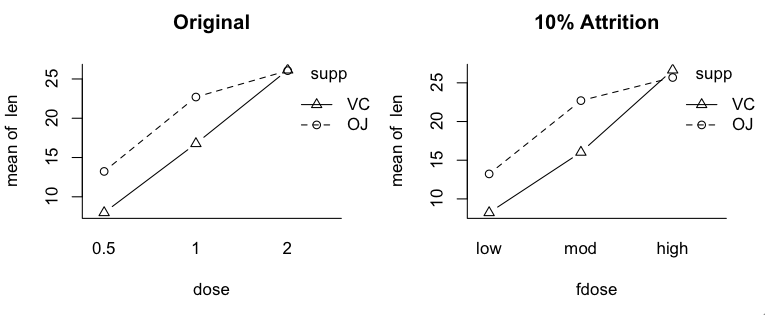
> source("aovIII.R")              # provided you have this in your working directory
> aovIII(len ~ supp * fdose, data=TG)
Single term deletions

Model:
len ~ supp * fdose
           Df Sum of Sq     RSS    AIC F value    Pr(>F)
<none>                   633.68 144.98
supp        1    169.71  803.40 155.79 12.8554 0.0007857 ***
fdose       2   2216.41 2850.10 222.17 83.9442 < 2.2e-16 ***
supp:fdose  2    141.96  775.65 151.89  5.3767 0.0078163 **
---
Signif. codes:  0 '***' 0.001 '**' 0.01 '*' 0.05 '.' 0.1 ' ' 1
We caught a bit of a break here with the significant interaction. Since that's
the effect of interest now, it's not so important how the main effects were
tested, but just out of curiosity, let's look at the Type II table anyway
(which I got by the trick of running the Type I tests twice with the factors
reversed).
            Df Sum Sq Mean Sq F value   Pr(>F)
supp         1  164.3   164.3  12.445 0.00093 ***
fdose        2 2215.8  1107.9  83.921 < 2e-16 ***
supp:fdose   2  142.0    71.0   5.377 0.00782 **
Residuals   48  633.7    13.2
---
Signif. codes:  0 '***' 0.001 '**' 0.01 '*' 0.05 '.' 0.1 ' ' 1
The differences are small, one might even be inclined to say trivial, so even
in the presence of a highly significant interaction, and with a more than minor
amount of subject attrition, the Type II and Type III tests are performing just
about the same. I'd cite the Type III tests here, but it's a moot point. It's
the simple effects we should now be interested in.
The question is over how to test the simple effects. It seems to me, if we are working on the pretext of equal cell weights when we do the omnibus ANOVA, then we should do the same when we test simple effects. I don't know of any way in R to wholly automate this. Perhaps that's for the best! Perhaps we need to do a little thinking for ourselves. I assume the following would be correct, and I'm sure if it isn't that I
will soon be hearing from someone who will set me straight. You'll know as
soon as I do!
Loneliness Parris Claytor (Psyc 497 Fall 2011) collected data from two surveys that she
administered via an online survey system (Sona). One survey was the
Embarrassability Scale (Modigliani, A. 1968. Embarrassment and embarrassability.
Sociometry, 31(3), 313-326), which measures susceptibility to being
embarrassed. The other was the Emotional-Social Loneliness Inventory
(Vincenzi, H. and Grabosky, F. 1987. Measuring the emotional/social aspects of
loneliness and isolation. Journal of Social Behavior & Personality, 2(2),
pt.2, 257-270), which measures emotional and social isolation (a score for each).
She was interested in seeing if the scores for embarrassability were positively
correlated with those for social isolation and emotional isolation. Her data can
be retrieved as follows:
Any of the three types of tests will show that the interaction is not
significant but also is not trivial (F > 1).
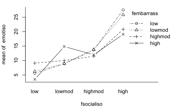
> aov.mod1 = aov(emotiso ~ fembarrass + fsocialiso, data=lone)
> summary(aov.mod1)
             Df Sum Sq Mean Sq F value   Pr(>F)
fembarrass    3    535   178.2   4.948  0.00298 **
fsocialiso    3   2756   918.8  25.507 1.79e-12 ***
Residuals   105   3782    36.0
---
Signif. codes:  0 '***' 0.001 '**' 0.01 '*' 0.05 '.' 0.1 ' ' 1

> aov.mod2 = aov(emotiso ~ fsocialiso + fembarrass, data=lone)
> summary(aov.mod2)
             Df Sum Sq Mean Sq F value   Pr(>F)
fsocialiso    3   3278  1092.6  30.332 3.33e-14 ***
fembarrass    3     13     4.4   0.123    0.946
Residuals   105   3782    36.0
---
Signif. codes:  0 '***' 0.001 '**' 0.01 '*' 0.05 '.' 0.1 ' ' 1
Now I'll point out that, if we had done Type II tests, we'd be looking at this
table right now.
             Df Sum Sq Mean Sq F value   Pr(>F)
fembarrass    3     13     4.4   0.123    0.946
fsocialiso    3   2756   918.8  25.507 1.79e-12 ***
Residuals   105   3782    36.0
NOTE: Or this one if you don't believe in dropping interactions. It doesn't
matter.
                      Df Sum Sq Mean Sq F value   Pr(>F)
fembarrass             3     13     4.4   0.130    0.942
fsocialiso             3   2756   918.8  26.973 9.72e-13 ***
fembarrass:fsocialiso  9    512    56.9   1.670  0.10677
Residuals             96   3270    34.1
And what would be lost? If I were reporting "main effects," this is the table that
I would report (i.e., the first one, since I'm a dropper), so in that sense,
nothing has been lost by just going straight
to the Type II tests. I'll also show you this.
> drop1(aov.mod1, test="F")
Single term deletions

Model:
emotiso ~ fembarrass + fsocialiso
           Df Sum of Sq    RSS    AIC F value    Pr(>F)
<none>                  3782.3 408.19
fembarrass  3     13.29 3795.6 402.59   0.123    0.9463
fsocialiso  3   2756.46 6538.7 463.50  25.507 1.787e-12 ***
---
Signif. codes:  0 '***' 0.001 '**' 0.01 '*' 0.05 '.' 0.1 ' ' 1

> drop1(aov.mod2, test="F")
Single term deletions

Model:
emotiso ~ fsocialiso + fembarrass
           Df Sum of Sq    RSS    AIC F value    Pr(>F)
<none>                  3782.3 408.19
fsocialiso  3   2756.46 6538.7 463.50  25.507 1.787e-12 ***
fembarrass  3     13.29 3795.6 402.59   0.123    0.9463
---
Signif. codes:  0 '***' 0.001 '**' 0.01 '*' 0.05 '.' 0.1 ' ' 1
The drop1() function reports the Type II tests no
matter which order the factors are in, and in either case, AIC is saying
"fembarrass" is not making an important contribution to the model. (Note: This
does not work from the full model, i.e., with the interaction included.)
I can't help pointing out though that, in the Type I tests, when "fembarrass" is entered first it is significant, and when it's entered second, it is not. When "fembarrass" is entered second, "socialiso" has gobbled up almost all of the variability once attributed to "fembarrass". I can't help wondering why. Hmmmm, let's think about that. Clearly, there is a relationship between "fembarrass" and "socialiso". Whatever could it be? Is it just an annoying confound of the kind we wish to get rid of when the data are experimental? Or is it nature trying to tell us something? If you've already read the Simple Mediation Analysis tutorial, then you already know my answer. But if you haven't, think about it a moment. Got it? Okay, here it is. I think embarrassability causes social isolation. When a person is easily embarrassed, he tends to avoid social situations where embarrassment might occur. Social isolation then causes a sense of emotional isolation (or loneliness). I'm proposing the following causal chain: "embarrass" -> "socialiso" -> "emotiso". If I'd been thinking traditional analysis of variance all along, and of course that means, with these data, Type II tests, I would have missed that entirely! Unless, of course, I'd stopped to think. And once I did that, I would have realized that Type I tests are the tests I want here. If my theory is true, then the Type I tests will show the pattern we have just seen. When the immediate cause is entered first, it "sucks all the life" out of the distant cause. When the distant cause is entered first, it claims that part of the variability it creates by acting through the immediate cause. The result is very similar to what we would see in a mediation analysis. The data are observational, of course, so the data alone cannot prove our hypothesized causal links. We need additional theoretical justification for that. But we have all the necessary relationships we would need to support the "causal chain" theory. The direct link between fembarrass and emotiso is strong, from fembarrass entered first (or entered only--it doesn't much matter). The indirect link between fembarrass and emotiso is weak to nonexistent, from fembarrass entered after fsocialiso. The link between fsocialiso and emotiso is strong even after fembarrass is removed, i.e., entered first. And finally, the link between fembarrass and fsocialiso is established by the fact that their effects change when the order in which they are entered is reversed. Despoilation of Movies You can hardly breathe these days without being exposed to advertising. TV has become all but unwatchable due to advertising, and yet we sit there glued to the set. The advertisers have a hook in our noses, and they know it. Better yet, for them, they have a hook in our kids' noses. Of course people complain about it, but they still buy the products, and that's all the advertisers care about. They don't care whether we like it or not as long as we're good little sheep spending our money. Even movies, which used to be more about the artistry, are now just another venue for advertising. Park and Berger (2010) studied the effectiveness of product placements in
movies by genre of film. They wanted to know how well viewers recalled products
they saw in movies depending upon whether the movie was an action flick, a comedy,
or a drama. The data can be obtained at the University of Florida Department of Statistics
website, and can be read directly into R as follows.
Now we have some work to do to get these data prepared. Specifically, we
need to make "gender" and "genre" into factors.
A good place to begin would be with an interaction plot.
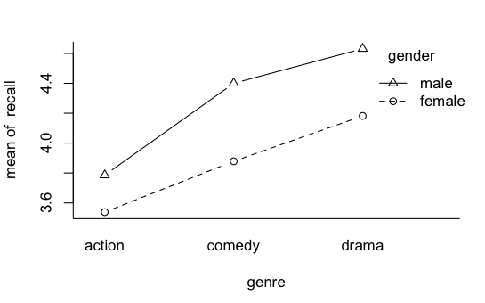
We should have already thought about this, but we didn't, so let's think at long last about how we're going to analyze this. The researchers did random assignment to genre and still managed to get a design way out of balance on that variable. On gender, which might be considered a blocking variable in this case, they apparently made no attempt to even get close to balance. Thus, we have a design which, for lack of a better word, I'll call "seriously" unbalanced. Given the cautions we've had about heterogeneity of variance in unbalanced
designs, we would do well to check.
What we want in this case from our main effects are traditional ANOVA main effects. I.e., we want what has been referred to as the "full benefit" of our factorial design. We want to see what the effect of genre is after we remove the confound with gender, and we want to see the effect of gender after we remove the confound with genre. How do we know that? Is there the possibility
of a natural relationship between genre and gender that we want to take into
account? Maybe if the researcher had let subjects choose the movies they wanted
to watch that would be the case. In fact, I suspect there would be a strong
relationship between gender and the kinds of movies men and women choose
to watch, but that's not how the study was set up. In this case, and relationship
we see between genre and gender is an undesirable confound. I would not hesitate
to choose Type II tests.
I have to wonder why this design wasn't balanced. What we essentially have here is a treatment by blocks design, with subjects randomly assigned to treatments but blocked by gender. Yet there are more than twice as many females as males. I get that if they took whoever volunteered, and their volunteers were coming from a pool of, say, psychology majors. Psych majors are generally predominantly female. But I'm sure these researchers had no intention of restricting their ability to generalize these results to psychology majors. Therefore, representing the population proportions in the cell frequencies is moot. Okay, so they took who they could get (volunteers), but they randomly assigned to genre. Why isn't the design at least balanced within genders (proportional balance)? The more I'm thinking about this, the more I'm thinking we want to analyze
as if the design were balanced. With this degree of imbalance, however,
I would do that very cautiously. Nevertheless, let's give it a shot just to see
what happens.
created 2016 February 28; updated 2016 March 25 |