
| Table of Contents
| Function Reference
| Function Finder
| R Project |
SIMPLE MEDIATION ANALYSIS
Preliminary Warning
Not an expert here! My knowledge of mediation analysis is rudimentary, so you
should take the word "simple" very seriously. I created this tutorial primarily
because I wanted to refer to it in the Unbalanced
Factorial Designs tutorial. If you want more details, I can recommend one
or more of the following references.
- Baron, R. M. and Kenny, D. A. (1986). The moderator-mediator variable
distinction in social psychological research: Conceptual, strategic, and
statistical considerations. Journal of Personality and Social Psychology,
51(6), 1173-1182.
- Hayes, A. F. and Preacher, K. J. (2014). Statistical mediation analysis with
a multicategorical independent variable. British Journal of Mathematical and
Statistical Psychology, 67, 451-470.
- Imai, K., Keele, L., and Tingley, D. (2010). A general approach to causal
mediation analysis. Psychological Methods, 15(4), 309-334.
- Imai, K., Keele, L., Tingley, D., and Yamamoto, T. (2015). Available at
CRAN as a PDF for download
here. (The link at Google Scholar to the original article
seems not to be working.)
- MacKinnon, D. P., Fairchild, A. J., and Fritz, M. S. (2007). Mediation
analysis. Annual Review of Psychology, 58.
- MacKinnon, D. P. and Fairchild, A. J. (2009). Current directions in
mediation analysis. Current Directions in Psychological Science, 18(1), 16-20.
- Rucker, D. D., Preacher, K. J., Tormala, Z. L., and Petty, R. E. (2011).
Mediation analysis in social psychology: Current practices and new recommendations.
Social and Personality Psychology Compass, 5/6, 359-371.
There are a couple of R optional packages at CRAN that perform mediation
analysis. The one most often referred to is called, simply enough, "mediation".
There is also a function in the "multilevel" package that will do simple
mediation analysis. I will not be referring to these packages in this tutorial.
My intent here is to show the basic process and logic of mediation, and I can
do that best, I think, using functions in the base R packages.
An Interesting Student Project
Parris Claytor (Psyc 497 Fall 2011) collected data from two surveys that she
administered via an online survey system (Sona). One survey was the
Embarrassability Scale (Modigliani, A. 1968. Embarrassment and embarrassability.
Sociometry, 31(3), 313-326), which measures susceptibility to being
embarrassed. The other was the Emotional-Social Loneliness Inventory
(Vincenzi, H. and Grabosky, F. 1987. Measuring the emotional/social aspects of
loneliness and isolation. Journal of Social Behavior & Personality, 2(2),
pt.2, 257-270), which measures emotional and social isolation (a score for each).
She was interested in seeing if the scores for embarrassability were positively
correlated with those for social isolation and emotional isolation. Her data can
be retrieved as follows:
> file = "http://ww2.coastal.edu/kingw/statistics/R-tutorials/text/loneliness.csv"
> lone = read.csv(file)
> dim(lone)        # note: one case was deleted due to missing values
[1] 112   5
> summary(lone)
   embarrass        socialiso     emotiso        fembarrass   fsocialiso
 Min.   : 32.00   Min.   : 0   Min.   : 0.00   high   :28   high   :24
 1st Qu.: 52.75   1st Qu.: 2   1st Qu.: 5.75   highmod:26   highmod:22
 Median : 65.00   Median : 6   Median :11.00   low    :28   low    :33
 Mean   : 64.90   Mean   : 7   Mean   :12.07   lowmod :30   lowmod :33
 3rd Qu.: 76.25   3rd Qu.:10   3rd Qu.:16.00
 Max.   :111.00   Max.   :31   Max.   :40.00
The first three variables, the scores from the scales mentioned above, are the
ones of interest to us. We can check to see if they are correlated easily
enough.
> cor(lone[,1:3])
          embarrass socialiso   emotiso
embarrass 1.0000000 0.4173950 0.2875657
socialiso 0.4173950 1.0000000 0.6397209
emotiso   0.2875657 0.6397209 1.0000000
 R does not give significance information with its correlation matrices
(annoying), but reference to a handy table will show that the critical value
of Pearson's r for a two-tailed test with 100 degrees of freedom (we have
df=110) is 0.254. Thus, all of these correlations surpass the .01 level of
significance. Parris's hypotheses were confirmed. The variables are positively
correlated.
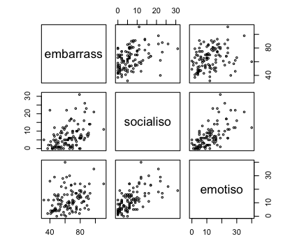
One more thing we should do is take a quick look at the
scatterplots to make sure the relationships are reasonably linear and that,
therefore, the above correlations are reasonable representions of the true
relationships among the variables.
> pairs(lone[,1:3], cex=.5)
Those graphs appear at right. They appear to show reasonably linear
relationships. All in all, it was an interesting project, especially to
someone like me who happens to have a special interest in shyness and
loneliness. I think we can take the analysis a bit further. This is
in no way a criticism of Parris's analysis. We don't teach mediation analysis
in any of the stat classes we offer in our program and, therefore, she had
not been exposed to it. Nevertheless, Parris has taken the first necessary
step in a mediation analysis, which is to show that the variables of
interest are, in fact, related to one another.
The Mediation Analysis
I think the sense of "emotional isolation" is a large part of loneliness.
I have a theory. My theory is that the "effect" of embarrassability on emotional
isolation/loneliness is not direct. I propose that there is a causal chain of
events that goes like this: high embarrassability leads the person to socially
isolate himself or herself, and this in turn causes a sense of emotional
isolation and loneliness. In other words, I am proposing the following causal
chain: embarrassability -> social isolation -> emotional isolation. Is there any
way to support this theory from these data?
We cannot demonstrate cause-and-effect relationships from correlational data.
However, we can show that these data are consistent (or not consistent) with the
theory using a technique called mediation analysis. The logic of mediation
analysis is shown in the next diagram.
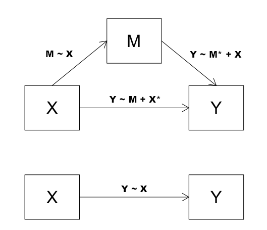
We observe a relationship between X and Y (bottom part of above diagram).
This relationship can be described by the regression relationship Y~X. In this
case, X is embarrassability and Y is emotional isolation. However, we believe
the real causal chain goes through a third variable, called a mediator variable
(also called an intervening variable), M, which in this case is social isolation.
The relationship between X and M can be described by the regression relationship
M~X, and between X and Y through M by the relationship Y~M+X, where we will look
particularly at the slope for M as an indicator of how strong the link is
between M and Y (after any effect of X has been removed). The relationship
between X and Y with M removed is also described by the regression relationship
Y~M+X, where we will look particularly at the slope for X as an indicator of how
strong this link is after M has been accounted for.
Let's get those regression coefficients.
> Model.1 = lm(emotiso~embarrass, data=lone)               # Y ~ X
> summary(Model.1)$coef   # we only need the coefficients
             Estimate Std. Error   t value    Pr(>|t|)
(Intercept) 2.5324683 3.11489671 0.8130184 0.417963731
embarrass   0.1469753 0.04667326 3.1490263 0.002109405

> Model.2 = lm(emotiso~socialiso+embarrass, data=lone)     # Y ~ M + X
> summary(Model.2)$coef
              Estimate Std. Error   t value     Pr(>|t|)
(Intercept) 5.75443805 2.54407898 2.2618944 2.568749e-02
socialiso   0.78450390 0.10094494 7.7716024 4.609403e-12
embarrass   0.01271865 0.04138834 0.3073004 7.592011e-01

> Model.3 = lm(socialiso~embarrass, data=lone)             # M ~ X
> summary(Model.3)$coef
              Estimate Std. Error   t value     Pr(>|t|)
(Intercept) -4.1070156 2.37085628 -1.732292 8.602452e-02
embarrass    0.1711357 0.03552464  4.817382 4.682879e-06
I'll add those coefficients to the diagram. NOTE: If you downloaded the
tutdata.zip file that comes with these tutorials (see
About The Data Sets), then you should have a function that will create
this diagram. It is an adaptation of a function that appeared in Wright and
London's textbook (see Refs). If you unzipped the
data folder and put it in your working directory, you can source in the
function and use it like this:
> source("tutdata/mediate.R")
> with(lone, mediate(embarrass,emotiso,socialiso,
+    names=c("embarrassability","emotional isolation","social isolation")))
       a        b        c       cp  sobel.z        p
0.171136 0.784504 0.146975 0.012719 4.070274 0.000047
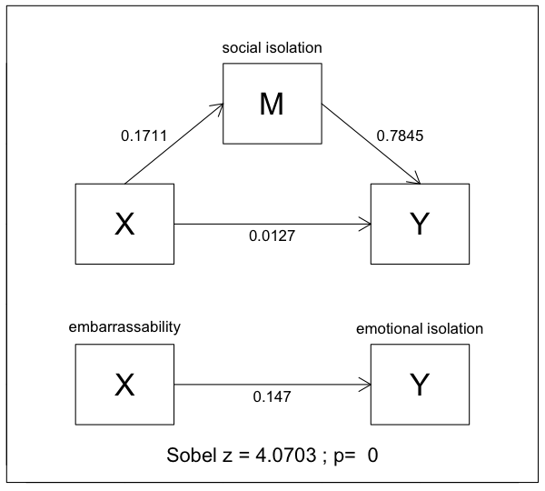
There are three kinds of results we can see from a simple mediation analysis:
no mediation, partial mediation, and complete mediation.
If there is no mediation, that means none of the effect is going through the
mediator variable. In the case of no mediation, the coefficients on the "straight
through" (X->Y) pathways in the two parts of the diagram would be about the
same, both 0.147 in this example. If there is partial mediation, the coefficient
on the "straight through" path in the top part of the diagram would be reduced
somewhat, the amount depending upon the strength of the mediation effect (more
reduction, stronger mediation effect). If there is complete mediation, the
coefficient on the "straight through" path in the top part of the diagram would
be reduced virtually to zero, indicating that all of the effect is going through
the mediator.
In this example, it's pretty clear that we have virtually complete
mediation of the effect of embarrassability on emotional isolation by the
intervening variable of social isolation. In the second regression analysis,
the effect of embarrassability on emotional isolation is not significant with a
slope of nearly zero, coef=.0127, p=.76. That is, when the mediator social
isolation is in the mix, it completely usurps the effect, leaving virtually
nothing for embarrassability to explain directly (or for other potential
mediators to explain, although this is a tricker conclusion).
Once again I emphasize that this does not demonstrate a causal link between
these variables. It is correlational data, after all. However, this is the
pattern we would expect to see if there is a causal link through the mediation
pathway, and therefore, this result is consistent with the theory I proposed.
A statistical test on the mediation effect (H0: there is no mediation effect)
is given by the z.value statistic in the output. This test statistic is called
Sobel's z, and is evaluated against a standard z-table.
The z statistic is calculated by first calculating the indirect effect,
which is the difference between the two values on the "straight through" paths.
Curiously enough, this value is also equal to the product of the two coefficients
on the sloped arrows in the diagram.
> .146975 - .012719
[1] 0.134256
> .171136 * .784504
[1] 0.1342569
This value is then divided by its estimated standard error. There is not uniform
agreement in the literature as to how this standard error should be calculated,
but the differences are small. In this case, the standard error is calculated
as follows, from regression coefficients and standard errors found in the
regression outputs for the values on the sloped paths.
> summary(Model.2)$coef
              Estimate Std. Error
(Intercept) 5.75443805 2.54407898
socialiso   0.78450390 0.10094494   <- this one (b, seb)
embarrass   0.01271865 0.04138834
> summary(Model.3)$coef
              Estimate Std. Error
(Intercept) -4.1070156 2.37085628
embarrass    0.1711357 0.03552464   <- and this one (a, sea)

> a = 0.1711357; sea = 0.03552464
> b = 0.78450390; seb = 0.10094494
> sqrt(a^2 * seb^2 + b^2 * sea^2 + sea^2 * seb^2)     # standard error calculation
[1] 0.03298467
> 0.134256 / 0.03298467                               # Sobel's z
[1] 4.070254
> pnorm(4.07, lower=F) * 2                            # two-tailed p-value
[1] 4.701314e-05
Indicating that the value on the top "straight through" pathway has been
significantly reduced from the value on the bottom "straight through" pathway.
You should be aware that this p-value should be considered approximate. To
make it reasonably accurate, we should have NO LESS than 50 cases in our
analysis, and 100 would be better (the more the merrier as they say). We have
N=112, so we can consider the p-value reasonable.
Another requirement of mediation analysis is that the causal chain go in
only one direction, from X towards Y. If there is any strange reciprocal
causation (say, Y influencing M), then mediation analysis may give an
incorrect result.
Mediation analysis also works if X is a factor, in which case it could be
considered a variation of ANCOVA.
Relationship to Other Methods
As I said, I wrote this tutorial because I wanted to refer to it from other
tutorials. So here is where I point out how other methods can give similar
information. I'm not suggesting that these methods are substitutes for the
above method, only that they can supply similar, if partial, information
about the mediation process.
Partial Correlation
There is no function for partial correlation in the R base packages.
However, there are optional packages with such functions (package "ppcor"
comes to mind), and several such functions have been made available on the
Internet. I'll use one posted at the Georgia Tech website of Soojin Yi that has
the advantage of being easy to source in. First, I'll look at a correlation
between "embarrass" and "emotiso" (which, in fact, we've already done), and
then I'll look at the partial correlation between those two variables after
"socialiso" has been removed.
> source("http://www.yilab.gatech.edu/pcor.R")
> with(lone, cor(embarrass, emotiso))
[1] 0.2875657
> with(lone, pcor.test(embarrass, emotiso, socialiso))
    estimate   p.value statistic   n gn  Method            Use
1 0.02942129 0.7586148 0.3073004 112  1 Pearson Var-Cov matrix
Pearson's r between the two variables is 0.288, but after "socialiso" is
removed, the partial correlation is only 0.029, which is no longer significantly
different from 0, p = .759. (I don't know what most of the stuff is in the
output. There is a webpage explaining it
here.)
Hierarchical Regression
Notice that we are comparing two regression models:
Model.1: lm(formula = emotiso ~ embarrass, data = lone)
Model.2: lm(formula = emotiso ~ socialiso + embarrass, data = lone)
In the first model, we put "embarrass" in alone. In the second model we put it
in along with "socialiso". Superficially, this resembles a hierarchical
regression, except in this case we're interested in what happens to the first
variable after the second one is added.
To find out what we want to know from a "proper" hierarchical regression,
we'd have to enter the variables the other way around, i.e., with the causally
prior variable entered first (the mediator).
> lm.soc = lm(emotiso ~ socialiso, data=lone)
> lm.socplusemb = lm(emotiso ~ socialiso + embarrass, data=lone)
And then we would compare the two models.
> anova(lm.soc, lm.socplusemb)
Analysis of Variance Table

Model 1: emotiso ~ socialiso
Model 2: emotiso ~ socialiso + embarrass
  Res.Df    RSS Df Sum of Sq      F Pr(>F)
1    110 4178.7
2    109 4175.1  1    3.6171 0.0944 0.7592
Presumably, we've already established a relationship between "embarrass" and
"emotiso", and now we're seeing that when "embarrass" is added after "socialiso",
it's effect disappears. In fact, R-squared hardly changes as all.
> summary(lm.soc)
... some output omitted ...
Residual standard error: 6.163 on 110 degrees of freedom
Multiple R-squared:  0.4092,	Adjusted R-squared:  0.4039
F-statistic:  76.2 on 1 and 110 DF,  p-value: 3.136e-14

> summary(lm.socplusemb)
... some output omitted ...
Residual standard error: 6.189 on 109 degrees of freedom
Multiple R-squared:  0.4098,	Adjusted R-squared:  0.3989
F-statistic: 37.83 on 2 and 109 DF,  p-value: 3.321e-13
The F test given in the output of anova() is a
test of this change in R-squared.
Type I Sums of Squares
You may have heard somewhere that the aov()
function in R does sequential tests. That is, in the following tests...
> print(summary(aov(emotiso ~ socialiso + embarrass, data=lone)), digits=6)
             Df  Sum Sq  Mean Sq  F value     Pr(>F)
socialiso     1 2894.75 2894.750 75.57438 4.0184e-14 ***
embarrass     1    3.62    3.617  0.09443     0.7592
Residuals   109 4175.06   38.303
---
Signif. codes:  0 '***' 0.001 '**' 0.01 '*' 0.05 '.' 0.1 ' ' 1
... "socialiso" is entered first, ignoring "embarrass", following which
"embarrass" is entered with any variability accounted for by the first variable
already removed from the DV. The total SS (i.e., the SS of the dependent
variable) is correctly partitioned, so finding the total SS is a matter of
adding.
> 2894.75 + 3.62 + 4175.06
[1] 7073.43
Thus, entering "socialiso" first yields an R-squared value of...
> 2894.75 / 7073.43
[1] 0.4092428
... and entering "embarrass" after "socialiso" increases R-squared by...
> 3.62 / 7073.43
[1] 0.0005117743
To within rounding error, that's what we saw in the hierarchical regression. (I
used print( , digits=6) to increase the precision
of the printed result.) Technical note: A more accurate version of this result
is 0.0005114, the square root of which is the semipartial correlation
between "embarrass" and "emotiso" with "socialiso" removed.
This method does not really establish all the links necessary to demonstrate
mediation, as it does not show the relationship between "embarrass" and "emotiso"
ignoring "socialiso", without which there would be nothing to mediate, and it
does not show the relationship between "embarrass" and "socialiso", a necessary
link on the mediation pathway. Both of those links can be demonstrated as
follows.
> print(summary(aov(emotiso ~ embarrass + socialiso, data=lone)), digits=6)
             Df  Sum Sq  Mean Sq F value     Pr(>F)
embarrass     1  584.93  584.930 15.2710 0.00016203 ***
socialiso     1 2313.44 2313.436 60.3978 4.6094e-12 ***
Residuals   109 4175.06   38.303
---
Signif. codes:  0 '***' 0.001 '**' 0.01 '*' 0.05 '.' 0.1 ' ' 1
Now we see that "embarrass" without (ignoring) "socialiso" has a considerable
link to "emotiso", R-squared = 584.93/7073.43 = 0.0827 (which is the square of
the correlation between "embarrass" and "emotiso"). We also see a substantial
link between "socialiso" and "emotiso" after "emabarrass" has been entered
(controlled, taken out), increase in R-squared = 2313.44/7073.43 = 0.327.
Finally, we see a substantial link between "embarrass" and "socialiso" in the
fact that the effects have changed so much when the order of entering the
variables was reversed. (In ANOVA we'd say the two explanatory variables are
confounded or nonorthogonal. In regression analysis we'd say they are
collinear.)
Is there enough information in these two tables to duplicate the mediation
analysis we did above? I suspect there is. In fact, intuitively I'd say there
has to be if someone wants to go to the trouble of ferreting it out, but it
would certainly be doing things the hard way!
What About Interactions?
I honestly don't know how mediation analysis would deal with an interaction
between the X variable and the mediator, but it seems to me it's something worth
checking for.
> print(summary(aov(emotiso ~ socialiso * embarrass, data=lone)), digits=6)
                     Df  Sum Sq  Mean Sq F value     Pr(>F)
socialiso             1 2894.75 2894.750 78.8278 1.6345e-14 ***
embarrass             1    3.62    3.617  0.0985   0.754244
socialiso:embarrass   1  209.04  209.039  5.6924   0.018779 *
Residuals           108 3966.02   36.722
---
Signif. codes:  0 '***' 0.001 '**' 0.01 '*' 0.05 '.' 0.1 ' ' 1
Uh oh! I will brazenly lift the following quote from
Dr. David A. Kenny's website. "Baron and Kenny (1986) and Kraemer et al.
(2002) discuss the possibility that M might interact with X to cause Y. Baron
and Kenny (1986) refer to this as M being both a mediator and a moderator and
Kraemer et al. (2002) as a form of mediation. The X with M interaction should
be estimated and tested and added to the model if present. Judd and Kenny (1981)
discuss how the meaning of path b [N.B., M->Y] changes when this interaction
is present." (References are given at Dr. Kenny's website.)
Beyond Simple Mediation
It has been argued that mediation analysis is better accomplished using the
method of structural equation modeling. Certainly, for models more complex than
the one above, SEM would have the advantage. See Iacobucci (2008) for a
summary of these methods. Parris Claytor's data and mediation will be discussed
again in the tutorial on Simple Path Analysis.
Also, there is a vignette on causal mediation analysis and the R mediation
package located here at
CRAN.
- Iacobucci, D. (2008). Mediation Analysis. Thousand Oaks, CA: Sage.
created 2016 March 22
| Table of Contents
| Function Reference
| Function Finder
| R Project |
|


 R does not give significance information with its correlation matrices
(annoying), but reference to a handy table will show that the critical value
of Pearson's r for a two-tailed test with 100 degrees of freedom (we have
df=110) is 0.254. Thus, all of these correlations surpass the .01 level of
significance. Parris's hypotheses were confirmed. The variables are positively
correlated.