
| Table of Contents
| Function Reference
| Function Finder
| R Project |
ANALYSIS OF COVARIANCE
Some people view ANCOVA as being a multiple
regression technique. Others see it as an offshoot of
ANOVA. In R, ANCOVA can be done with equal success using either the lm() function or the aov()
function. I find it easier to treat ANCOVA as regression, so that's what
I'll do.
Everything is regression, after all. The previous tutorial was called
Multiple Regression, and we treated only cases
where all the explanatory, or predictor, variables were numeric. It's possible
to include categorical predictors (IVs) if they are coded correctly. In fact,
if all we have are categorical IVs, then we are essentially doing ANOVA. If
there is a mix of numeric and categorical IVs, then we are in the realm
of ANCOVA.
Gas Mileage
A car with an eight cylinder engine... What teenaged boy hasn't dreamed of
owning one? Well, get one now before they become extinct, because they are
hard on gasoline! Of course, cars with big engines also tend to weigh more than
cars with smaller engines, so maybe it's not the number of cylinders in the
engine so much as it is the weight of the car that costs us at the gas pump. I
wonder how we might tease those two variables apart.
> names(mtcars)
 [1] "mpg"  "cyl"  "disp" "hp"   "drat" "wt"   "qsec" "vs"   "am"   "gear" "carb"
> cars = mtcars[,c(1,2,6)]
> cars$cyl = factor(cars$cyl)
> summary(cars)
      mpg        cyl          wt
 Min.   :10.40   4:11   Min.   :1.513
 1st Qu.:15.43   6: 7   1st Qu.:2.581
 Median :19.20   8:14   Median :3.325
 Mean   :20.09          Mean   :3.217
 3rd Qu.:22.80          3rd Qu.:3.610
 Max.   :33.90          Max.   :5.424
The "mtcars" data set contains information on cars that were road-tested by
Motor Trend magazine in 1974 (or road tests of which were published in
1974). That's a long time ago, unless you're me, and you're still dreaming of
that 1967 Mustang! It's the data we have, so we'll go with it. You can update
the data on your own time if you want to see if relationships we discover from
1974 still hold today.
We have extracted three columns from that data frame, namely, mpg (gas
mileage in miles per U.S. gallon), cyl (the number of cylinders in the engine),
and wt (weight in 1000s of pounds). The "cyl" variable has sensibly been declared
a factor. Let's begin by looking at some graphs.
> par(mfrow=c(1,3))
> boxplot(mpg ~ cyl, data=cars, xlab="cylinders", ylab="mpg")
> boxplot(wt ~ cyl, data=cars, xlab="cylinders", ylab="weight")
> plot(mpg ~ wt, data=cars)
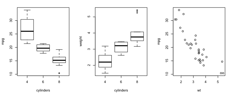 That doesn't leave much to the imagination, does it?! The more cylinders the
car has (had!), the harder it is on gas. The more cylinders the car has, the
more it weighs. And the more the car weighs, the lower its gas mileage. All
three of those relationships appear impressively strong in the graphs.
That doesn't leave much to the imagination, does it?! The more cylinders the
car has (had!), the harder it is on gas. The more cylinders the car has, the
more it weighs. And the more the car weighs, the lower its gas mileage. All
three of those relationships appear impressively strong in the graphs.
An analysis of variance will no doubt show us in p-values what we can
already plainly see from looking at the boxplots.
> lm.out1 = lm(mpg ~ cyl, data=cars)   # aov() works as lm() internally
> anova(lm.out1)                       # same as summary.aov(lm.out1)
Analysis of Variance Table

Response: mpg
          Df Sum Sq Mean Sq F value    Pr(>F)
cyl        2 824.78  412.39  39.697 4.979e-09 ***
Residuals 29 301.26   10.39
---
Signif. codes:  0 '***' 0.001 '**' 0.01 '*' 0.05 '.' 0.1 ' ' 1

> summary(lm.out1)

Call:
lm(formula = mpg ~ cyl, data = cars)

Residuals:
    Min      1Q  Median      3Q     Max
-5.2636 -1.8357  0.0286  1.3893  7.2364

Coefficients:
            Estimate Std. Error t value Pr(>|t|)
(Intercept)  26.6636     0.9718  27.437  < 2e-16 ***
cyl6         -6.9208     1.5583  -4.441 0.000119 ***
cyl8        -11.5636     1.2986  -8.905 8.57e-10 ***
---
Signif. codes:  0 '***' 0.001 '**' 0.01 '*' 0.05 '.' 0.1 ' ' 1

Residual standard error: 3.223 on 29 degrees of freedom
Multiple R-squared:  0.7325,	Adjusted R-squared:  0.714
F-statistic:  39.7 on 2 and 29 DF,  p-value: 4.979e-09
No surprises in the ANOVA output. The interesting stuff is in the regression
output. The (estimated) coefficients relate to the means of "cyl". The base, or
reference, level of "cyl" is the one not listed with a coefficient in the
regression output, or cyl4. The intercept (26.66) is the mean gas mileage for
that level of "cyl". The coefficient for cyl6 is -6.92, which means that six
cylinder cars get (got) 6.92 mpg less than four cylinder cars, on the average.
Eight cylinder cars got 11.56 mpg less than four cylinder cars. The significance
tests on these coefficients are equivalent to Fisher LSD tests on the differences
in means. These figures are easily enough confirmed. (Important note: This
interpretation of the coefficients depends upon having contrasts for unordered
factors set to "treatment". Do options("contrasts")
to check.)
> with(cars, tapply(mpg, cyl, mean))
       4        6        8
26.66364 19.74286 15.10000
The effect size is R2 = .7325. In the language of ANOVA, that
statistic would be called eta-squared. That is the "proportion of explained
variation" in mpg accounted for by the explanatory variable. I don't think
there's any doubt of a cause-and-effect relationship in this case (maybe a
wee bit), but this does not mean that number of cylinders explains the whole
73% of variability in gas mileage. A more accurate statement would be
cylinders and all confounds from other variables that might be confounded with
cylinders account for
73% of the variability in gas mileage. The last line of the regression
output duplicates the ANOVA output, because there is only one explanatory
variable at this time.
We think one of the variables confounded with cylinders is weight of the
vehicle. In fact, we think once those gas mileages are adjusted for the weight
of the vehicle, the differences in the means by number of cylinders will be a
lot less impressive. Dare we imagine that the differences might vanish
altogether? I don't think so. But, let's see. Now for the analysis of covariance
part.
> lm.out2 = lm(mpg ~ wt + cyl, data=cars)
> anova(lm.out2)
Analysis of Variance Table

Response: mpg
          Df Sum Sq Mean Sq  F value    Pr(>F)
wt         1 847.73  847.73 129.6650 5.079e-12 ***
cyl        2  95.26   47.63   7.2856  0.002835 **
Residuals 28 183.06    6.54
---
Signif. codes:  0 '***' 0.001 '**' 0.01 '*' 0.05 '.' 0.1 ' ' 1

> summary(lm.out2)

Call:
lm(formula = mpg ~ wt + cyl, data = cars)

Residuals:
    Min      1Q  Median      3Q     Max
-4.5890 -1.2357 -0.5159  1.3845  5.7915

Coefficients:
            Estimate Std. Error t value Pr(>|t|)
(Intercept)  33.9908     1.8878  18.006  < 2e-16 ***
wt           -3.2056     0.7539  -4.252 0.000213 ***
cyl6         -4.2556     1.3861  -3.070 0.004718 **
cyl8         -6.0709     1.6523  -3.674 0.000999 ***
---
Signif. codes:  0 '***' 0.001 '**' 0.01 '*' 0.05 '.' 0.1 ' ' 1

Residual standard error: 2.557 on 28 degrees of freedom
Multiple R-squared:  0.8374,	Adjusted R-squared:   0.82
F-statistic: 48.08 on 3 and 28 DF,  p-value: 3.594e-11
In the ANOVA, we have added "wt" (weight), a numeric variable that we think
(i.e., know perfectly well in this case) is related to the DV as a covariate.
Ordinarily, at least in the social sciences, we would do such a thing because
we think the covariate will help discriminate among levels of the categorical
IV, once the confound with the covariate is removed. Here we believe just the
opposite is going to occur. We're not so terribly interested in the relationship
between weight and gas mileage. We just want to get it out of the mix, so that
we can see a "purer" relationship between cylinders and gas mileage.
Two very important points need to be made at this juncture. First, notice
we didn't ask to see any interactions between "wt" and "cyl". That means we're
assuming there aren't any, a common assumption in ANCOVA, but also an assumption
that is commonly incorrect. It is worth checking. Second, in R, the ANOVA tests
are sequential. That means if we want weight taken out before we look at the
effect of cylinders, we MUST enter it first into the model formula. This won't
make any difference in the regression output, but it makes a BIG difference in
the ANOVA output!
Overall, we are now accounting for R2 = .8374, or 84% of the
total variability in gas mileage. However, notice that the part of the
explained variability that we can attribute to "cyl" (eta-squared for "cyl")
is now only...
> 95.26 / (847.73 + 95.26 + 183.06)
[1] 0.0845966
...or about 8%. The mighty have, indeed, fallen, but not so far that "cyl" is no
longer a statistically significant effect. Are there other confounds with "cyl"
that might remove that last 8%? I'll leave it up to you to look for them.
We can now calculate adjusted means of "cyl" by level. This is done
using the regression equation, and we have a different regression equation for
each of the three levels of "cyl".
mpg-hat = 33.9908 - 3.2056 * wt for cyl4
mpg-hat = 33.9908 - 3.2056 * wt - 4.2556 for cyl6
mpg-hat = 33.9908 - 3.2056 * wt - 6.0709 for cyl8
The terms for specific levels of "cyl" can be combined with, and thus will
change, the intercept of the regression line, and usually they are, but I have
left them separated here to illustrate what's happening. To get the adjusted
means for levels of "cyl", we fill in the overall average of "wt" and
solve each of these regression equations.
> mean(cars$wt)
[1] 3.21725
> 33.9908 - 3.2056 * mean(cars$wt)               # adjusted mean for cyl4
[1] 23.67758
> 33.9908 - 3.2056 * mean(cars$wt) - 4.2556      # adjusted mean for cyl6
[1] 19.42198
> 33.9908 - 3.2056 * mean(cars$wt) - 6.0709      # adjusted mean for cyl8
[1] 17.60668
Notice that the means are still different--and significantly different as we
can tell from the ANOVA--but not so different as they were before we took out
the effect of the weight of the car on gas mileage.
Here's a nice way to graph these results.
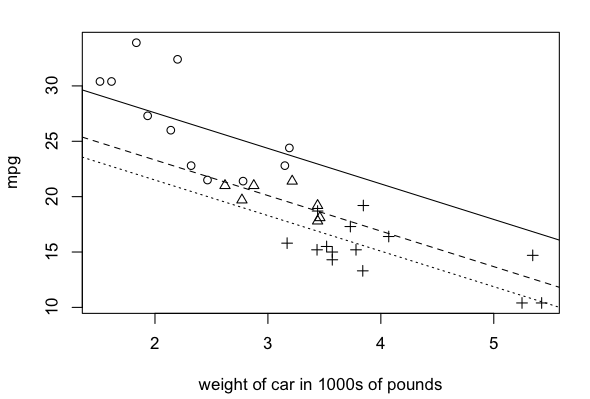
> plot(mpg ~ wt, data=cars, pch=as.numeric(cars$cyl), xlab="weight of car in 1000s of pounds")
> abline(a=33.99, b=-3.21, lty="solid")
> abline(a=33.99-4.26, b=-3.21, lty="dashed")
> abline(a=33.99-6.07, b=-3.21, lty="dotted")
The circles and solid line are for the four-cylinder cars, the triangles and
dashed line for the six-cylinder cars, and the plus symbols and dotted line for
the eight-cylinder cars. I'll refer you to the
More Graphics tutorial for instructions on how to add all that information to
the graph.
Two things distress me here that I feel compelled to comment on. First,
notice there is very little overlap on the scatterplot in the weight of 4- vs.
6- vs. 8-cylinder cars. This makes the calculation of adjusted means just a
little bit dicey. Also, while I don't detect anything obvious on the graph, I'm
still uncomfortable that we haven't checked for the possibility of interactions
between "wt" and "cyl".
> lm.out3 = lm(mpg ~ wt * cyl, data=cars)
> anova(lm.out2, lm.out3)
Analysis of Variance Table

Model 1: mpg ~ wt + cyl
Model 2: mpg ~ wt * cyl
  Res.Df    RSS Df Sum of Sq      F Pr(>F)
1     28 183.06
2     26 155.89  2     27.17 2.2658 0.1239
Interactions make no significant contribution to the model, but I'd be
happier if that F-value were closer to 1. (Note: This method of comparing
models is explained in the Multiple Regression
tutorial.)
An Aside
Above I noted that, in R, ANOVA is done sequentially, and that makes it
very important to get the covariate into the model formula first. If you don't
care for sequential sums of squares, you can try this, provided you have
installed the optional "car" package from CRAN. (See
Package Management.)
> library("car")                       # this will give an error if "car" is not installed
> Anova(lm.out2)                       # notice the upper case A in Anova
Anova Table (Type II tests)

Response: mpg
           Sum Sq Df F value   Pr(>F)
wt        118.204  1 18.0801 0.000213 ***
cyl        95.263  2  7.2856 0.002835 **
Residuals 183.059 28
---
Signif. codes:  0 '***' 0.001 '**' 0.01 '*' 0.05 '.' 0.1 ' ' 1
These are so-called Type II sums of squares, and they are not calculated
sequentially. I would hesitate to calculate eta-squares from this table
unless I got the total SS by some method other than adding the SSs in
this table. (See the tutorial on Unbalanced
Designs for a discussion.)
Childhood Abuse and Adult Post-Traumatic Stress Disorder
The data for this section of the tutorial is discussed in Faraway (2005).
To get the data, you can either install the "faraway" package, or you can go
to Dr.
Faraway's website and
download the data files that accompany his book. The files will download into
a folder called "jfdata.zip", which will unzip into a folder called "ascdata".
Rename this folder "Faraway" and drop it into your working directory (Rspace).
If you have installed the "faraway" package, the commands to get the data
are:
> library("faraway")
> data(sexab)
If you have downloaded the Faraway folder to your working directory, then do
this:
> sexab = read.table("Faraway/sexab.txt", header=T, row.names=1)
Either way...
> summary(sexab)
      cpa               ptsd               csa
 Min.   :-3.1204   Min.   :-3.349   Abused   :45
 1st Qu.: 0.8321   1st Qu.: 6.173   NotAbused:31
 Median : 2.0707   Median : 8.909
 Mean   : 2.3547   Mean   : 8.986
 3rd Qu.: 3.7387   3rd Qu.:12.240
 Max.   : 8.6469   Max.   :18.993
The data are from a study by Rodriquez, et al. (1997). The subjects were adult
women who were being treated at a clinic, some of whom self-reported childhood
sexual abuse (csa=Abused), and some of whom did not (csa=NotAbused). All of the
women filled out two standardized scales, one assessing the severity of
childhood physical abuse (cpa), and one assessing the severity of adult
post-traumatic stress disorder (ptsd). On both of these scales, a higher score
indicates a worse outcome. The question we will attempt to answer
is, How are sexual and physical abuse that occur in childhood related to the
severity of PTSD as an adult, and how does the effect of physical abuse differ
for women who were or were not sexually abused as children?
When I discuss this example in my class, I always start off by having
students examine the following scatterplot. (DON'T close this graphics window.
We will be drawing regression lines on this graph eventually.)
> plot(ptsd ~ cpa, data=sexab, pch=as.numeric(csa), col=as.numeric(csa))
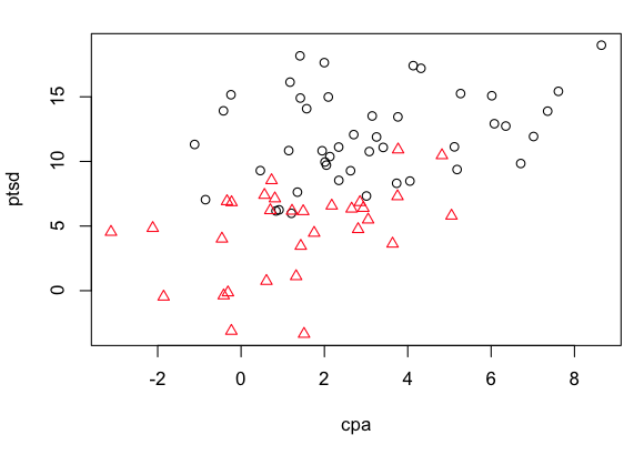 The red triangles are for women who were not sexually abused as children, and
the black open circles are for women who were. I ask my students to tell me
what they can see in this graph, and I hope against hope for the following
answers.
The red triangles are for women who were not sexually abused as children, and
the black open circles are for women who were. I ask my students to tell me
what they can see in this graph, and I hope against hope for the following
answers.
- There is a clear positive relationship between the severity of childhood
physical abuse and the severity of adult PTSD.
- Overall, women who were not sexually abused as children have lower severity
of adult PTSD than do women who were sexually abused as children.
- Overall, women who were not sexually abused as children also had lower
severity of physical abuse as children than did women who were sexually abused
as children.
Then I ask them the hard question. Does the effect of physical abuse add to the
effect of sexual abuse, or not? When we summarize the relationships we see on
this graph, and we going to have to do so with two regression lines, or will one
be sufficient? Let's find out.
First, I propose we check for the importance of interactions.
> lm.sexab1 = lm(ptsd ~ cpa + csa, data=sexab)
> lm.sexab2 = lm(ptsd ~ cpa * csa, data=sexab)
> anova(lm.sexab1, lm.sexab2)
Analysis of Variance Table

Model 1: ptsd ~ cpa + csa
Model 2: ptsd ~ cpa * csa
  Res.Df    RSS Df Sum of Sq     F Pr(>F)
1     73 782.08
2     72 774.28  1    7.8069 0.726  0.397
I like that. The F-value is near 1, so we can assume the absence of important
interactions. That will make our analysis easier.
> anova(lm.sexab1)                     # sequential tests
Analysis of Variance Table

Response: ptsd
          Df Sum Sq Mean Sq F value    Pr(>F)
cpa        1 449.80  449.80  41.984 9.462e-09 ***
csa        1 624.03  624.03  58.247 6.907e-11 ***
Residuals 73 782.08   10.71
---
Signif. codes:  0 '***' 0.001 '**' 0.01 '*' 0.05 '.' 0.1 ' ' 1

> summary(lm.sexab1)

Call:
lm(formula = ptsd ~ cpa + csa, data = sexab)

Residuals:
    Min      1Q  Median      3Q     Max
-8.1567 -2.3643 -0.1533  2.1466  7.1417

Coefficients:
             Estimate Std. Error t value Pr(>|t|)
(Intercept)   10.2480     0.7187  14.260  < 2e-16 ***
cpa            0.5506     0.1716   3.209  0.00198 **
csaNotAbused  -6.2728     0.8219  -7.632 6.91e-11 ***
---
Signif. codes:  0 '***' 0.001 '**' 0.01 '*' 0.05 '.' 0.1 ' ' 1

Residual standard error: 3.273 on 73 degrees of freedom
Multiple R-squared:  0.5786,	Adjusted R-squared:  0.5671
F-statistic: 50.12 on 2 and 73 DF,  p-value: 2.002e-14
We have an answer. The estimated coefficient for csaNotAbused is
statistically significant. When we include it in the regression equation(s),
it will result in different intercepts for the csaAbused and csaNotAbused
lines. Furthermore, the difference in intercepts, 6.3 points on a scale with
a range of scores of a little more than 22 points, is quite large. The
regression equations are:
ptsd-hat(Abused) = 10.2480 + 0.5506 * cpa
ptsd-hat(NotAbused) = 10.2480 + 0.5506 * cpa - 6.2728 = 3.9752 + 0.5506 * cpa
To draw the regression lines on the pre-existing scatterplot...
> abline(a=10.25, b= 0.55, lty="dashed", col="black")
> abline(a=3.98, b=0.55, lty="dotted", col="red")
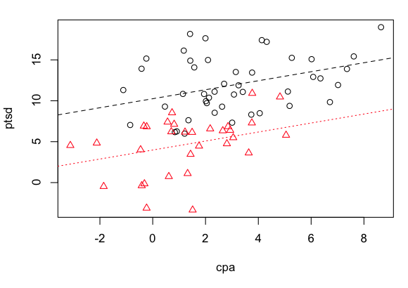 It appears that the effects of physical and sexual abuse are additive. One does
not make the effects of the other more severe (no interaction), which is in no way
to say that they aren't each bad enough to begin with!
Same Aside
It appears that the effects of physical and sexual abuse are additive. One does
not make the effects of the other more severe (no interaction), which is in no way
to say that they aren't each bad enough to begin with!
Same Aside
Here are the Type II (nonsequential) tests from the "car" package.
> Anova(lm.sexab1)
Anova Table (Type II tests)

Response: ptsd
          Sum Sq Df F value    Pr(>F)
cpa       110.30  1  10.295  0.001982 **
csa       624.03  1  58.247 6.907e-11 ***
Residuals 782.08 73
---
Signif. codes:  0 '***' 0.001 '**' 0.01 '*' 0.05 '.' 0.1 ' ' 1
This changes nothing in the regression analysis, as regression effects are
not calculated sequentially.
- Rodriguez, N., Ryan, S. W., Vande Kemp, H., & Foy, D. W. (1997).
Posttraumatic stress disorder in adult female survivors of childhood sexual
abuse: A comparison study. Journal of Counseling and Clinical Psychology, 65,
53-59.
created 2016 February 18
| Table of Contents
| Function Reference
| Function Finder
| R Project |
|