> ls()
[1] "bygroups"  "sampsize"  "sem"       "SS"        "summarize"
> getwd()                              # just checking!
[1] "/Users/billking/Rspace"
> save.image("myfunctions.RData")
> rm(list=ls())
> ls()
character(0)

Making a Modification or Two

I'm not entirely happy with our sampsize() function. First of all, I don't like the name. I also don't like that, as the length() function does, it does things its way and offers us no opportunity to modify that. What I want is a length function with an na.rm option.

Open a script window (File > New Script in Windows or File > New Document on a Mac), and type this.

size = function(X, na.rm=TRUE)
{
   ifelse(na.rm,
      length(X) - sum(is.na(X)),
      length(X))
}

> size(rivers)
[1] 141
> size(1:100)
[1] 100
> size(c(1:98,NA,NA))
[1] 98
> length(c(1:98,NA,NA))
[1] 100
> size(c(1:98,NA,NA), na.rm=F)
[1] 100

> load("myfunctions.RData")
> rm(sampsize)
> save.image("myfunctions.RData")

summarize = function(X)
{
	c(MEAN=mean(X, na.rm=T),
	  MEDIAN=median(X, na.rm=T),
	  SD=sd(X, na.rm=T),
	  N=length(X)-sum(is.na(X)),
	  NAs=sum(is.na(X)))
}

> summarize(rivers)
    MEAN   MEDIAN       SD        N      NAs 
591.1844 425.0000 493.8708 141.0000   0.0000 
> summarize(c(1:100))
     MEAN    MEDIAN        SD         N       NAs 
 50.50000  50.50000  29.01149 100.00000   0.00000 
> summarize(c(1:98,NA,NA))
    MEAN   MEDIAN       SD        N      NAs 
49.50000 49.50000 28.43413 98.00000  2.00000 
> summarize(c(1:98,NA,NA,1000))
    MEAN   MEDIAN       SD        N      NAs 
59.10101 50.00000 99.62936 99.00000  2.00000

> save.image("myfunctions.RData")      # good idea to ls() it first!
> rm(list=ls())

Error Bars, Critical r, and Cohen's d

In this and future sections of this tutorial, I am going to be typing my functions into a script window. That way they will be much easier to fix if (when!) I screw them up. Reminder: The script window is reached in Windows via File > New Script, and on a Mac via File > New Document.

There is no facility in R for plotting error bars on bar graphs (or any other kind of graph). Putting on my R apologist hat, I would say fine, because bar graphs are for frequencies, not for means! But not everyone sees it that way, and I must respect their right to be mistaken, so I'm told. So here is an error.bars() function. If you want to just copy and paste it into R to create the function, I'm okay with that.

error.bars = function (x, y, e, cbl = 0.03) 
{
    num.groups = length(x)
    for (i in 1:num.groups) {
        arrows(x[i], y[i] - e[i], x[i], y[i] + e[i], angle = 90, 
            length = cbl, code = 3)
    }
}

Bar graphs are tricky in R, because they don't plot bars where you might expect to find them. Let me show you.

> summary(chickwts)                              # some data to demonstrate
     weight             feed   
 Min.   :108.0   casein   :12  
 1st Qu.:204.5   horsebean:10  
 Median :258.0   linseed  :12  
 Mean   :261.3   meatmeal :11  
 3rd Qu.:323.5   soybean  :14  
 Max.   :423.0   sunflower:12  
> means = with(chickwts, tapply(weight, feed, mean))       # get and save means
> barplot(means)
> barplot(means, ylim=c(0,500))                            # make room for error bars
> sds = with(chickwts, tapply(weight,feed, sd))            # get and save SDs
> lengths = with(chickwts, tapply(weight, feed, length))   # get and save Ns
> sems = sds / sqrt(lengths)                               # get sems
> barplot(means, ylim=c(0,500)) -> bp                      # I always forget this!
> bp                                             # this is where the bars are plotted!
     [,1]
[1,]  0.7
[2,]  1.9
[3,]  3.1
[4,]  4.3
[5,]  5.5
[6,]  6.7
> error.bars(x=bp, y=means, e=sems, cbl=.1)      # draw the error bars

> ls()
[1] "bp"         "error.bars" "lengths"    "means"      "sds"        "sems"      
> rm(bp, lengths, means, sds, sems)
> ls()
[1] "error.bars"

r.crit = function (df, alpha = 0.05) 
{
    t1 = qt(p = alpha, df = df, lower.tail = FALSE)
    r1 = sqrt(t1^2/(t1^2 + df))
    t2 = qt(p = alpha/2, df = df, lower.tail = FALSE)
    r2 = sqrt(t2^2/(t2^2 + df))
    output = c(df, alpha, r1, r2)
    names(output) = c("df", "alpha", "1-tail", "2-tail")
    output = round(output, 4)
    output
}

> cor(USArrests)
             Murder   Assault   UrbanPop      Rape
Murder   1.00000000 0.8018733 0.06957262 0.5635788
Assault  0.80187331 1.0000000 0.25887170 0.6652412
UrbanPop 0.06957262 0.2588717 1.00000000 0.4113412
Rape     0.56357883 0.6652412 0.41134124 1.0000000
> dim(USArrests)
[1] 50  4
> r.crit(df=48, alpha=.01)                  # default alpha is .05
     df   alpha  1-tail  2-tail 
48.0000  0.0100  0.3281  0.3610

Cohens.d = function(group1, group2)
{
   group1 = group1[!is.na(group1)]          # strip NAs from group 1
   group2 = group2[!is.na(group2)]          # strip NAs from group 2
   SSE = var(group1)*(length(group1)-1)+var(group2)*(length(group2)-1)
   dfE = length(group1)+length(group2)-2
   MSE = SSE/dfE
   pooled.s = sqrt(MSE)
   diff = abs(mean(group1)-mean(group2))
   t = diff/(pooled.s*sqrt(1/length(group1)+1/length(group2)))
   c(diff=diff,t=t,Cohens.d=abs(mean(group1)-mean(group2))/pooled.s)
}

> casein = chickwts$weight[chickwts$feed=="casein"]
> horsebean = chickwts$weight[chickwts$feed=="horsebean"]
> Cohens.d(horsebean, casein)
      diff          t   Cohens.d 
163.383333   7.019741   3.005674

> ls()
[1] "casein"     "Cohens.d"   "error.bars" "horsebean"  "r.crit"    
> rm(casein, horsebean)
> ls()                                           # can't be too safe!
[1] "Cohens.d"   "error.bars" "r.crit"    
> load("myfunctions.RData")                      # add the previous ones
> ls()                                           # really! you can't be too safe!
[1] "bygroups"   "Cohens.d"   "error.bars" "r.crit"     "sampsize"   "sem"       
[7] "SS"         "summarize" 
> save.image("myfunctions.RData")                # save all of them
> rm(list=ls())

Some Functions Related to ANOVA

With apologies to Red Green, what's the difference between Type III sums of squares and a trampoline? You take your shoes off to jump on a trampoline! Type III sums of squares are the bane of ANOVA with unbalanced designs. At least, you'd get that impression from listening to the R community. (See the tutorial on unbalanced designs for details.) But sometimes you just got to have them. Bill Venables, a staunch critic of Type III, let the cat out of the box as to how to get them in R. Here is a function.

aovIII = function (formula, data = NULL) 
{
  options(contrasts = c("contr.sum", "contr.poly"))
  aovIII.out <<- aov(formula, data)
  print(drop1(aovIII.out, . ~ ., test = "F"))
  options(contrasts = c("contr.treatment", "contr.poly"))
}

> data(genotype, package="MASS")                 # get some unbalanced data
> summary(genotype)                              # weight of crossfostered mice by litter and mother
 Litter Mother       Wt       
 A:17   A:16   Min.   :36.30  
 B:15   B:14   1st Qu.:48.20  
 I:14   I:16   Median :54.00  
 J:15   J:15   Mean   :53.97  
               3rd Qu.:60.30  
               Max.   :69.80  
> with(genotype, table(Litter,Mother))           # check the cell frequencies
      Mother
Litter A B I J
     A 5 3 4 5
     B 4 5 4 2
     I 3 3 5 3
     J 4 3 3 5
> aovIII(Wt ~ Mother * Litter, data=genotype)    # the Type III tests
Single term deletions

Model:
Wt ~ Mother * Litter
              Df Sum of Sq    RSS    AIC F value  Pr(>F)  
<none>                     2440.8 257.04                  
Mother         3    671.74 3112.6 265.87  4.1282 0.01142 *
Litter         3     27.66 2468.5 251.73  0.1700 0.91612  
Mother:Litter  9    824.07 3264.9 256.79  1.6881 0.12005  

> summary(aovIII.out)                            # the Type I tests
              Df Sum Sq Mean Sq F value  Pr(>F)   
Mother         3  771.6  257.20   4.742 0.00587 **
Litter         3   63.6   21.21   0.391 0.76000   
Mother:Litter  9  824.1   91.56   1.688 0.12005   
Residuals     45 2440.8   54.24

> rm(genotype, aov.outIII)

rmsaov.test = function(matname) 
{
    s <- dim(matname)[1]
    df.subjects <- s - 1
    a <- dim(matname)[2]
    df.treatment <- a - 1
    total.df <- a * s - 1
    total.SS <- var(as.vector(matname)) * total.df
    treatment.SS <- var(margin.table(matname, 2)) * df.treatment/s
    treatment.MS <- treatment.SS/df.treatment
    subjects.SS <- var(margin.table(matname, 1)) * df.subjects/a
    subjects.MS <- subjects.SS/df.subjects
    error.SS <- total.SS - treatment.SS - subjects.SS
    df.error <- df.treatment * df.subjects
    error.MS <- error.SS/df.error
    STATISTIC <- treatment.MS/error.MS
    PARAMETER <- c(df.treatment, df.error)
    PVAL <- pf(STATISTIC, df.treatment, df.error, lower.tail = FALSE)
    DNAME <- deparse(substitute(matname))
    METHOD <- "Oneway ANOVA with repeated measures"
    names(STATISTIC) <- "F"
    names(PARAMETER) <- c("df treat", "df error")
    OUT <- list(statistic = STATISTIC, parameter = PARAMETER, 
        p.value = PVAL, method = METHOD, data.name = DNAME, MS.treatment = treatment.MS, 
        MS.error = error.MS, MS.subjects = subjects.MS)
    class(OUT) <- "htest"
    print(OUT)
    print(c(MS.error = error.MS, MS.treat = treatment.MS, MS.subjs = subjects.MS))
    cat("\n")
    cat("Treatment Means\n")
    print(apply(matname, 2, mean))
    cat("\n")
    cat("Compound Symmetry Check (Variance-Covariance Matrix)\n")
    covmat <- cov(matname)
    print(covmat)
    cat("\n")
    cat("Estimated Greenhouse-Geisser Epsilon and Adjusted p-value\n")
    D <- a^2 * (mean(diag(covmat)) - mean(covmat))^2
    N1 <- sum(covmat^2)
    N2 <- 2 * a * sum(apply(covmat, 1, mean)^2)
    N3 <- a^2 * mean(covmat)^2
    epsilon <- D/((a - 1) * (N1 - N2 + N3))
    p.adj <- pf(treatment.MS/error.MS, df.treatment * epsilon, 
        df.error * epsilon, lower.tail = FALSE)
    GGE <- c(epsilon, p.adj)
    names(GGE) = c("epsilon", "p-adjust")
    print(GGE)
}

Here are two examples of how to use this function. The first one involves fetching some data from a help page for Friedman's test (a nonparametric repeated measures ANOVA). The data are base running times for three different methods of rounding first base. (The help page contains some errors, but see for more details.)

> example(friedman.test)                    # output not shown; but there's a lot!
> ls()
[1] "aovIII"        "rmsaov.test"   "RoundingTimes" "wb"
> head(RoundingTimes)                       # the data matrix we are after
  Round Out Narrow Angle Wide Angle
1      5.40         5.50       5.55
2      5.85         5.70       5.75
3      5.20         5.60       5.50
4      5.55         5.50       5.40
5      5.90         5.85       5.70
6      5.45         5.55       5.60
> class(RoundingTimes)                      # it must be a matrix
[1] "matrix"
> rmsaov.test(RoundingTimes)

	Oneway ANOVA with repeated measures

data:  RoundingTimes
F = 6.2883, df treat = 2, df error = 42, p-value = 0.004084

   MS.error    MS.treat    MS.subjs 
0.007451299 0.046856061 0.200887446 

Treatment Means
   Round Out Narrow Angle   Wide Angle 
    5.543182     5.534091     5.459091 

Compound Symmetry Check (Variance-Covariance Matrix)
              Round Out Narrow Angle Wide Angle
Round Out    0.07387987   0.06310065 0.06327922
Narrow Angle 0.06310065   0.06747294 0.06705628
Wide Angle   0.06327922   0.06705628 0.07443723

Estimated Greenhouse-Geisser Epsilon and Adjusted p-value
    epsilon    p-adjust 
0.773501463 0.008439799

> rm(RoundingTimes, wb)                     # clean up a bit first
> data(anorexia, package="MASS")            # fetch the data
> head(anorexia)
  Treat Prewt Postwt
1  Cont  80.7   80.2
2  Cont  89.4   80.1
3  Cont  91.8   86.4
4  Cont  74.0   86.3
5  Cont  78.1   76.1
6  Cont  88.3   78.1
> class(anorexia)                           # this is no good!
[1] "data.frame"
> anor = as.matrix(anorexia[,2:3])          # convert the relevant columns to a matrix
> rmsaov.test(anor)

	Oneway ANOVA with repeated measures

data:  anor
F = 8.6293, df treat = 1, df error = 71, p-value = 0.004458

 MS.error  MS.treat  MS.subjs 
 31.86892 275.00694  59.55305 

Treatment Means
   Prewt   Postwt 
82.40833 85.17222 

Compound Symmetry Check (Variance-Covariance Matrix)
          Prewt   Postwt
Prewt  26.85796 13.84207
Postwt 13.84207 64.56401

Estimated Greenhouse-Geisser Epsilon and Adjusted p-value
    epsilon    p-adjust 
1.000000000 0.004457718

> ls()
[1] "anor"        "anorexia"    "aovIII"      "rmsaov.test"
> rm(anor, anorexia)                        # get rid of the junk
> ls()                                      # check!
[1] "aovIII"      "rmsaov.test"
> load("myfunctions.RData")                 # add the functions in myfunctions
> ls()                                      # check again!
 [1] "aovIII"      "bygroups"    "Cohens.d"    "error.bars"  "r.crit"      "rmsaov.test"
 [7] "sampsize"    "sem"         "SS"          "summarize"  
> save.image("myfunctions.RData")           # save a new myfunctions file
> rm(list=ls())                             # clean up
> ls()
character(0)

Linear Contrasts

There is no easy way in the base R packages to test complex linear contrasts. So we're going to create one. The method of calculation will be based on that in the very excellent statistics book The Statistical Sleuth (3rd ed.) by Ramsey and Schafer (2013).

t.contrast = function(means,codes,n,spool,dfe)
{
  g = sum(means*codes)
  seg = spool*sqrt(sum(codes^2/n))
  t = g/seg
  p.value = pt(abs(t),dfe,lower.tail=FALSE)*2
  d = abs(g/spool)
  output <<- c(g=g,SE=seg,t=t,df=dfe,p.value=p.value,d=d)
  round(output,4)
}

This is how the function works. Linear contrasts are used as an alternative to ANOVA and are sometimes referred to as planned comparisons. ANOVA is a fine tool, but it tests an alternative hypothesis that is very general, i.e., any pattern of means other than all means equal. Thus, ANOVA is most appropriate when you don't really know much about what to expect from your treatments. If you have specific hypotheses, for example, group A will have a higher mean than group B, and groups B and C will be the same, then planned comparisons are more appropriate.

> ls()                       # your workspace should contain only the function
[1] "t.contrast"
> data(chickwts)             # weights of chickens by type of feed they received
> summary(chickwts)
     weight             feed   
 Min.   :108.0   casein   :12  
 1st Qu.:204.5   horsebean:10  
 Median :258.0   linseed  :12  
 Mean   :261.3   meatmeal :11  
 3rd Qu.:323.5   soybean  :14  
 Max.   :423.0   sunflower:12

We need to feed our t.contrast function five pieces of information: a vector of group means, a vector of contrast codes, a vector of group sizes (can be one number if the design is balanced), the pooled standard deviation calculated over all groups, and the degrees of freedom for error, which is total number of subjects minus the number of groups they've been divided into if the design is between groups. Let's start getting that stuff.

> means = with(chickwts, tapply(weight,feed,mean))
> codes = c(1/2, -1/4, -1/4, -1/4, -1/4, 1/2)         # best entered as fractions
> n = c(12, 10, 12, 11, 14, 12)                       # from the summary above
> aov(weight~feed, data=chickwts)                     # easiest way to get spool
Call:
   aov(formula = weight ~ feed, data = chickwts)

Terms:
                    feed Residuals
Sum of Squares  231129.2  195556.0
Deg. of Freedom        5        65

Residual standard error: 54.85029

> spool = 54.85029                                    # it's the residual s.e.
> dfe = 65

> t.contrast(means, codes, n, spool, dfe)
       g       SE        t       df  p.value        d 
100.6781  13.7969   7.2972  65.0000   0.0000   1.8355

Now let's add the function to our file. First, make sure there is nothing in your workspace except this function.

> ls()
[1] "chickwts"   "codes"      "dfe"        "means"      "n"         
[6] "output"     "spool"      "t.contrast"
> rm(chickwts, codes, dfe, means, n, output, spool)
> ls()
[1] "t.contrast"

> load("myfunctions.RData")
> ls()
 [1] "aovIII"      "bygroups"    "Cohens.d"    "error.bars"  "r.crit"      "rmsaov.test"
 [7] "sampsize"    "sem"         "SS"          "summarize"   "t.contrast" 
> save.image("myfunctions.RData")
> rm(list=ls())

There is one more thing I want to do to prepare us for the next section of this tutorial.

> data(anorexia, package="MASS")       # we'll use this below
> save.image("anorexia.RData")         # a saved project
> rm(anorexia)                         # clean up
> palm483S = rnorm(50)                 # some junk for the workspace

Putting It All Together and Using It

We now have eleven shiny new functions in a file called myfunctions.RData. In my case, I have this file saved to my Rspace directory, because that's usually where I go to do my R work. You should adjust the advice here to fit your own working habits.

When I start R, I immediately change my working directory to Rspace. Then I examine my workspace, and if there is stuff there I don't want, I remove it. I load anything from Rspace that I might be working on. Then I'm ready to go to work.

Suppose I wanted to use one or more of the functions we've just created. It's an RData file, so I could load() it, but that would put all those functions in my workspace, and I don't want that. So instead of loading it, I'm going to attach it to the search path. My work flow might look like this.

> setwd("Rspace")                      # don't do this if you're already in Rspace
> ls()
[1] "palm483S"
> rm(palm483S)
> attach("myfunctions.RData")

> search()
 [1] ".GlobalEnv"             "file:myfunctions.RData" "tools:RGUI"            
 [4] "package:stats"          "package:graphics"       "package:grDevices"     
 [7] "package:utils"          "package:datasets"       "package:methods"       
[10] "Autoloads"              "package:base"          
> ls(pos=2)
 [1] "aovIII"      "bygroups"    "Cohens.d"    "error.bars"  "r.crit"      "rmsaov.test"
 [7] "sampsize"    "sem"         "SS"          "summarize"   "t.contrast"

> dir()                                # see what's in Rspace
[1] "anorexia.RData"    "myfunctions.RData" "UCB.RData"
> load("anorexia.RData")               # load the previously saved project I want
> ls()                                 # nobody here but us data sets
[1] "anorexia"
> head(anorexia)
  Treat Prewt Postwt
1  Cont  80.7   80.2
2  Cont  89.4   80.1
3  Cont  91.8   86.4
4  Cont  74.0   86.3
5  Cont  78.1   76.1
6  Cont  88.3   78.1
> dim(anorexia)
[1] 72  3
> with(anorexia, cor(Prewt, Postwt))   # do some analysis
[1] 0.3324062
> r.crit(df=70)                        # use one of our custom functions
     df   alpha  1-tail  2-tail 
70.0000  0.0500  0.1954  0.2319 
> bygroups(data=anorexia$Postwt, groups=anorexia$Treat)    # use another one
     CBT     Cont       FT 
85.69655 81.10769 90.49412
> summarize(anorexia$Prewt)                                # caught me again; this is the old one
     mean        SD         N 
82.408333  5.182466 72.000000
> detach("file:myfunctions.RData")     # done with it; get it out of the search path

Review of Steps For Modifying Your Functions File

You may want to add a function of your own to this file, or delete one. Or you may want to modify one of these functions. Just to collect the steps together in a neat outline, here's how you would do it. Make sure the file is not attached to your search path before you begin.

To delete a function (or a data object that snuck in there somehow):

• Change to the working directory that has the myfunctions.RData file in it.
• Clear your workspace.
• load("myfunctions.RData")
• Remove the undesired function or functions from your workspace using rm().
• save.image("myfunctions.RData")
• Clear your workspace.

To add a function:

• Change to the working directory that has the myfunctions.RData file in it.
• Clear your workspace.
• Write the new function in the script editor (or in a text editor) and read it into R (Execute or Run All from the script window, or copy and paste). I.e., get it into your workspace, and make sure it's the ONLY thing in your workspace.
• Make sure the new function doesn't have the same name as an old one, or it will be overwritten at the next step.
• load("myfunctions.RData")
• save.image("myfunctions.RData")
• Clear your workspace.

To modify a function:

• Change to the working directory that has the myfunctions.RData file in it.
• Clear your workspace.
• load("myfunctions.RData")
• Type the name of the function you wish to modify at the command prompt without parentheses. This will print the definition of the function to your Console. Example:
  

  > aovIII
  function (formula, data = NULL, subset=NULL) 
  {
    options(contrasts = c("contr.sum", "contr.poly"))
    aov.out <<- aov(formula, data, subset)
    print(drop1(aov.out, . ~ ., test = "F"))
    options(contrasts = c("contr.treatment", "contr.poly"))
  }

• Copy and paste the function definition to your script window and insert the function name and an = sign before the word function. (NOTE: You can also try fix(aovIII), which may or may not work. In this case, DO NOT type in the function name =.)
• Make the desired mods. For example, if you don't want aovIII to save the aov.out object to your workspace, modify the aov.out <<- line to aov.out <-.
• Read the modified function into R (or close the window opened by fix and choose Save).
• save.image("myfunctions.RData")
• Clear your workspace.

I should also note that you can add other objects, such as data frames, vectors, matrices, etc., to this file if you want to keep them there for some reason. I have a long list of data frames in mine that I use in my teaching. Sending the file to my students by e-mail is a convenient way to get a large number of data files to them. (No, I won't send it to you. Some of the data files were collected by students and are not for public use. Sorry.)

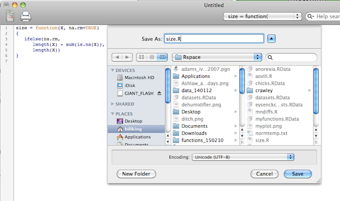
An Alternative Method

If you don't really need all your scripts and data files in one big file such as myfunctions.RData, then it may be more convenient to just save them a script at a time in your working directory (Rspace). Open a script window, type the script, then save it with a convenient name and .R as the extension. Be sure R is saving it to your working directory. This is not the default in the script editor, at least not on the Mac, so make the necessary changes in the dialogue box before saving.

Then when you need to use it, you just source it in.

> setwd("Rspace")
> source("size.R")
> size(c(NA,1:5,NA,NA,NA))
[1] 5