R Tutorials--More and Fancier Graphics

MORE AND FANCIER GRAPHICS

Preliminaries

If you use it for nothing else, you should consider using R as your graphics engine. In up-to-date installations of R, the "graphics" library loads by default when R is started, so you should be ready to go as soon as R opens. It's possible to set up R in such a way that this is not the case, however. So if you are working with someone else's R installation, and graphics is not working, try this.

> library(graphics)                    # In any event, this does no harm.

Another command you may find handy is...

> par(ask=T)                           # Do this now! (It will open a graphics device.)

This command will cause R to pause between printing out graphs and ask you (in the Console window) to hit the Enter key. Usually, the message will be "Waiting to confirm page change". When you see this message, R is telling you it is waiting to print a graphic, and that you should press Enter to allow it to happen. (The Console window must have focus. Click in it if not.) If "ask=" is set to FALSE, and R has multiple graphics to print, they will fly by on your monitor so fast you will not be able to see them! (It's annoying otherwise, so you may want to set "ask=" to FALSE after you run the following demos.)

Now, for just a taste of what R is capable of graphics-wise, try running these commands in the R Console (output not shown here).

> example(plot)                        # Remember to press Enter when prompted.
> example(barplot)                     # Some are better than others!
> example(boxplot)
> example(dotchart)
> example(coplot)
> example(hist)
> example(fourfoldplot)
> example(stars)
> example(image)
> example(contour)
> example(filled.contour)
> example(persp)                       # Saving the best for last!

This will fill your workspace with all kinds of stuff, so clean up before going on. And set par(ask=F).

Those are many, but not quite all, of the high level graphics functions in the R base packages that are loaded by default at start-up. There is also a package called "lattice" that does lattice graphics and can be loaded with the library(lattice) command if needed. Other packages contain some graphics functions as well. Try truehist() in the MASS package.

Some, but not all, of the options that can be set within many of these functions are:

col= - set or change the color of something
legend= - add a legend (T or F)
lty= - set the line type ("solid", "dashed", "dotted")
lwd= - set the line width (thickness)
main= - set the main title at the top of the graph
pch= - set the character for plotted points (1 through 20)
xlab= - set the label on the x-axis
ylab= - set the label on the y-axis
xlim= - set the numeric limits on the x-axis
ylim= - set the numeric limits on the y-axis

See the help pages for details. Finally, here is a list of some, but not all, of the low level graphics functions that are available for modifying a graph after it has been drawn.

abline() - draw lines
arrows() - draw arrows
axis() - draw an axis
curve() - draw a curve (also high level, use add=T)
legend() - create a custom legend
lines() - draw lines and points
points() - draw lines and points
text() - add text
title() - add a main title or x,y-axis labels

Some Graphics Basics

For the real basics, see the Describing Data Graphically tutorial, which you probably should read first if you are not familiar with high-level vs. low-level graphics functions, etc.

In R, when you issue a high level plotting command, R will open a graphics window (which in R-speak is called a "device") if one is not already open. This window will have certain defaults. It will be 7 in. by 7 in. (672x672 pixels) in size. It will use a 12-point sans serif font for text. And so on. For example...

> ### Close any open graphics windows before doing this.
> plot(pressure)

To take personal control of the graphics window, close the graphics window now open on your monitor, and try this.

In Windows

> windows(width=5, height=4, pointsize=18)
> plot(pressure)

You will notice windows() removes focus from the R Console, so you will have to click in the Console window to continue working. Also, the function is NOT window(), which does something different. You are asking for the Windows graphics device.

On the Mac

> quartz("Quartz", width=5, height=4, pointsize=18)
> plot(pressure)

You will notice quartz() removes focus from the R Console, so you will have to click in the Console window to continue working. The first argument in this function is the name you would like the graphics window to have. This is annoying, if you ask me, because what do I care what the name of the window is? I always use "Quartz" or "Q". The name MUST be present nevertheless. Remember this command, by the way, if you have an old MacBook, because the default 7x7 in. graphics device is too big to display on the old MacBook screen.

In Linux

> x11(display=" ", width, height, pointsize)

I have yet to get this to work in Linux, so I have just given the syntax of the command. According to the help page, the default for the "display=" option is the value in the user's enivornment variable DISPLAY, but this is NOT the case. There is NO DEFAULT, and a value must be specified inside the function. No matter what I enter there, it just doesn't work!

All Users

See the help file for the OS-specific command above for more options that can be set. You can open multiple graphics devices at once, if you have some need for that. All graphics devices can be closed like this.

> graphics.off()

The current graphics device can be closed with dev.off(). You can also see a list of currently open graphics devices with dev.list(). To illustrate...

> graphics.off()                       # Turn off all graphics devices to begin.
> windows(5, 5, 18)                    # On the Mac: quartz("Quartz", 5, 5, 18)
> plot(eruptions~waiting, data=faithful)
> title(main="Old Faithful Data")
> windows(7, 3, 10)                    # On the Mac: quartz("Quartz", 7, 3, 10)
> plot(eruptions~waiting, data=faithful)
> title(main="Old Faithful Data in Another Format")
> windows(6, 5, 14)                    # On the Mac: quartz("Quartz", 6, 5, 14)
> boxplot(decrease~treatment, data=OrchardSprays)
> title(main="Orchard Sprays Data")
> dev.list()                           # See a list of open devices.
windows windows windows                ### This is in Windows. Output will
      2       3       4                ### be different in other OSes.
> dev.off()                            # Close the current device.
windows 
      2 
> graphics.off()                       # Close 'em all.

The function plot.new() will also open a new graphics window and will paint in the default background color. There are no options for setting window size with this command, however. If you have your graphics window set up for multiple plots (see below), plot.new() can be used to skip a panel.

Writing Graphics Output Directly to a File

When you are getting a complex graphic ready for publication, the best way to go about it is to write your commands in a script. You can open the script editor from the menu in the R Console GUI (unless you are in a terminal in Linux or in the Mac terminal) and write your commands there. These commands can then be executed over and over from the editor menu and edited until you get them just the way you want. Then what?

At this point, you may want to write your graphics output directly to a file. The following simple example will illustrate how this is done.

> setwd("Rspace")            # if you haven't already and have this directory
> png(filename="myplot.png", width=500, height=500, pointsize=10)
> plot(pressure)
> title(main="Vapor pressure of Mercury")
> dev.off()                  ### This is crucial!
null device 
          1

The first line of this example changes your working directory to Rspace, if you are still in the default working directory. The graphic will be written to your working directory, whatever you have that set to. If you want it to go somewhere else, you can give a full pathname. The second line opens a file for output of a graphic in PNG format. This is a good format for graphics with few colors in them. On the Mac, it's a handy thing to be able to do, since from the pulldown menus on the Mac graphics device, the only format in which files can be saved is PDF. (You can always screenshot it. That's what I do.) For graphics with subtle shades of color in them, use jpeg() instead of png(). Other formats available are tiff() and bmp(). The first option gives the filename. Then the width and height of the plot are given in pixels (default is 480 by 480, which is not the same as the default graphics device). Finally, the pointsize of the font is given (default is 12).

After this command is issued, all further graphics output is sent to this file. Finally, the dev.off() function writes and closes the file. DON'T FORGET TO DO THIS! See the help page for more options that can be set. You can also write out graphics files using pdf() and postscript(). However, the function syntax is different, and you should consult the help pages before using these functions. PDF files can be very nice since they are scalable, but postscript files are not as useful on Windows or Mac systems. Both of these OSes will convert them to PDF before displaying them.

Interacting With a Graph

There are add-on packages that allow you to do amazing things with R plots, including rotate them in three dimensions. I'm not familiar with them, so I will stick to the two basic R functions that allow you to interact with plots: locator() and identify().

First, let's get a plot to work with.

> boxplot(decrease ~ treatment, data=OrchardSprays)   # output not shown

If you execute this command in R, you will see a series of boxplots labeled A through H on the horizontal axis. There are three outliers, for treatments A, C, and G. Suppose we want to identify the data values that correspond to a couple of those outlying points. There are a number of ways to do it, but I'll do it by interacting with the plot using the locator() function. A warning in advance: This function returns the coordinates of a mouse click made on a graph. It does NOT return the coordinates of a data point. So by clicking on these points, we will get the APPROXIMATE data values. Second warning: locator() will remain active until it locates as many mouse clicks as you asked for, or until you tell it to stop. How you tell it to stop can be difficult (for me) to remember, and is operating system dependent. So BE SURE you give it a number as an argument when you use this function. It works like this.

> locator(n=2)                    # we're good to go for two mouse clicks
> ### click in the graphics window to bring it to focus, then click on the points (Mac)
$x                                # possible values from perfectly aimed clicks are 1, 2, 3,..., 8
[1] 2.996876 6.996876

$y                                # these should both be whole numbers as well
[1] 84.04680 24.18964

After you issue the command in the R Console, the current graphics device window will come into focus (not on the Mac--you'll have to click in the graphics window), and your mouse pointer will turn into a little crosshair. Center the crosshair over the point you want to identify and click the left mouse button. Nothing will happen, except maybe an audio cue. Click on the other point (you've asked to identify two points) and R will return information about those points. (Default is 512 points! In Windows, there is a "Stop" menu in the graphic device window when you initiate this function, so you can stop at any time by using that menu.) On the first line of the printout is the x-coords of the points you clicked on (not interesting in this case, except to identify which boxplot you're looking at), and on the second line are the y-coords of those points. Once again, these are NOT the exact data values of the points, but if you were careful, they should be pretty close. This would have been the more sensible ways to get the actual data values...

> with(OrchardSprays, tapply(decrease, treatment, range))  ## output not shown

...but I wanted to illustrate the function. The locator() function can also be used to plot points on a graph and do draw lines between plotted points or mouse clicks. You can read the help page to see how that works. In my opinion, the most useful aspect of this function is for putting text or other elements on the graph exactly where you want them.

Suppose we want to label those two points with their values (which are 84 and 24). We can use text() to add text to an existing graph, but text() has to be fed x- and y-coordinates, and this can involve some guesswork. Or we could do this.

> text(locator(1),"84")                # Now click where you want the center of the label.
> text(locator(1),"24")                # And click again next to the proint.

The text inside the quotes will be added to the graph, CENTERED on your mouse click (so click where you want the CENTER of the label). A bit later we'll use this trick to add legends to graphs.

The identify() function is a bit tricker. And as is often the case in R, the help page is of very little help until after someone actually explains to you how the function works! And furthermore, R people, your example is atrocious! Even Murrell (2006), the best source on R graphics I know of, shies away from explaining this function, stating merely that the "function can be used to add labels to data symbols on a plot. The data point closest to the mouse click gets labelled" (p. 41). Well, often it doesn't, and often when it does the label is not placed in a very sensible location. I haven't found the function very useful, and I would suggest that using locator() is a much better way of labeling points.

All that having been said, the identify() function can be useful for identifying data points in scatterplots, especially when the data are from a data frame with rownames.

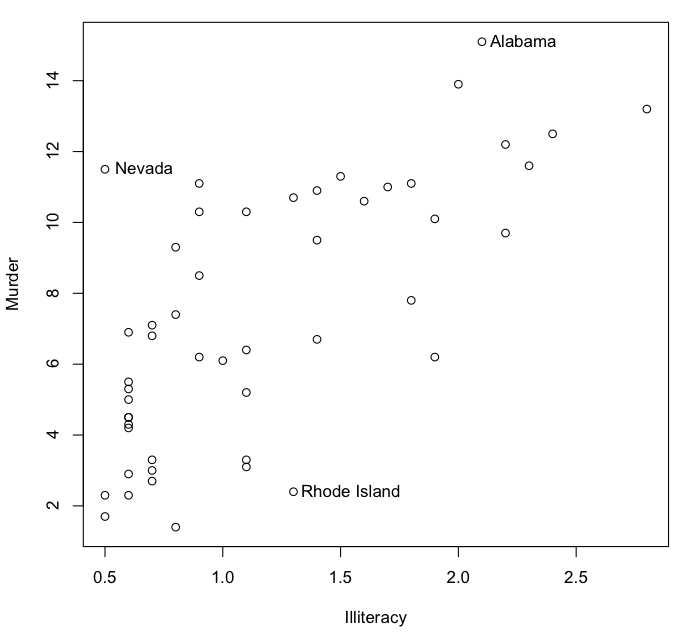
> state.data = as.data.frame(state.x77)     # convert data set state.x77 from matrix to dataframe
> plot(Murder ~ Illiteracy, data=state.data)

As you can see, there is a distinct positive relationship between illiteracy and murder rate. Now do this.

> identify(x=state.data$Illiteracy, y=state.data$Murder,
+          labels=rownames(state.data), atpen=T, n=3)

R is now waiting for you to click near any 3 data points on the scatterplot. When you do, the points will be labeled with the name of the state. (If we hadn't specified "labels=", the labels would be the index number of the case in the data frame.) THIS IS IMPORTANT: Because we set atpen=T, the lower left corner of the label will be placed at the click location. So be careful where you click. This is the only way I've been able to get the labels plotted in sensible locations! This will work unless the point is too near the right side of the plot. You could rescale the x-axis to leave room for any such labels. By the way, "x=" specifies the x-coords of the plotted points, "y=" specifies the y-coords, "labels=" is a character vector of labels to be used, and "n=" specifies the number of points to be labeled (default is the number of values in x).

Adding Legends

Some high level plotting functions in R have an option for adding a legend. For example...

> data.table = margin.table(Titanic, c(2,1))
> barplot(data.table, beside=T, legend=T)        # output not shown

Convenient, but wouldn't it be nice if we could put that legend in the upper left corner of the graph rather than in the upper right corner where it overlaps one of the bars? We can.

There is a function called legend() that allows you to customize the legend to your heart's content (and then some). Let's start the graph over again.

> graphics.off()                       # or just click it away
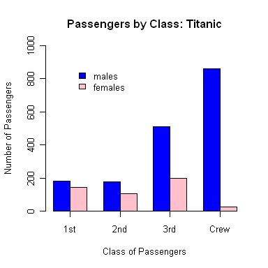
> windows(4, 4, 10)                    # on a Mac: quartz("Quartz", 4, 4, 10)
> barplot(data.table,                  # you can put all this on one line
+         beside=T,                    # plot the bars side by side
+         axis.lty=1,                  # get an x-axis with ticks
+         ylim=c(0,1000),              # set scale of y-axis
+         col=c("blue","pink"))        # it is important to know the colors used
> title(xlab="Class of Passengers",
+       ylab="Number of Passengers")   # label the axes
> title(main="Passengers by Class: Titanic")     # add a main title

And now for the legend.

> legend(locator(1),                   # we will place it with a mouse click
+        legend=c("males","females"),  # the text to be used in the legend
+        fill=c("blue","pink"),        # the colors to fill legend boxes
+        bty="n")                      # turn off putting a box around legend

R is now waiting for you to click somewhere on the graph. Click where you want the upper left corner of the legend leaving a bit of allowance for the fact that normally the legend will have a box around it. Some notes: You can also specify "x=" and "y=" if you know the xy-coordinates where you want the legend placed. The default is to draw a box around the legend, but just to be cute, I turned it off in this example. The legend() function has a very large number of options, and I can't explain them all here. See the help page and experiment! The useful options will vary depending upon what kind of graph you have, but at least this example will get you started.

This will give you some idea of what's possible.

> graphics.off()
> example(legend)
> rm(list=ls())

I turned off your graphics device to begin with to start with fresh plots. There are a good many examples, so don't forget to press the Enter key when you get the prompt to do so. Finally, this makes a mess in your workspace, so I cleaned it out at the end, but you may want to be more circumspect if there is stuff there you want to keep (hopefully not too late to remind you of this). The only caution I have about legends is to know what colors and symbols are being used in your plots, because you will have to duplicate them in the legend.

This is where R's color palettes may come in handy. R will keep track of the colors for you. Let's redraw that last graph.

> barplot(data.table,                  # you can put all this on one line
+         beside=T,                    # plot the bars side by side
+         axis.lty=1,                  # get an x-axis with ticks
+         ylim=c(0,1000),              # set scale of y-axis
+         col=rainbow(2))              # use a color palette
> title(xlab="Class of Passengers",
+       ylab="Number of Passengers")
> title(main="Passengers by Class: Titanic")

This time instead of asking for specific colors, we let R choose them by specifying a color palette called "rainbow" and telling it how many colors we wanted (2). To add the appropriate legend, we do the same thing.

> legend(x=2, y=890,                   # use xy-coords (found with locator())
+        legend=c("males","females"),  # as before
+        fill=rainbow(2))              # as in the barplot() command

This time I included the default box around the legend, and I used xy-coords to place the legend, not because I had to, but to illustrate those options. Color palettes available include rainbow, heat.colors, terrain.colors, topo.colors, and cm.colors. Although not technically a color palette, you can also use gray or grey. The syntax is a bit different, so see the help page. All of these color palette names are functions, so be sure to use them as such.

Finally, here is that first graph as a script, in case you want to play. Typing a long, delicate sequence of commands like this into a script window is a very good idea, in case you screw up and have to start over. Also, you can save the script to a file and reload it later if you decide to make changes.

quartz("Quartz", 4, 4, 10)            # change this for Windows
barplot(data.table,                   # you can put all this on one line
         beside=T,                    # plot the bars side by side
         axis.lty=1,                  # get an x-axis with ticks
         ylim=c(0,1000),              # set scale of y-axis
         col=c("blue","pink"))        # it is important to know the colors used
title(xlab="Class of Passengers",
       ylab="Number of Passengers")   # label the axes
title(main="Passengers by Class: Titanic")     # add a main title

legend(locator(1),                    # we will place it with a mouse click
        legend=c("males","females"),  # the text to be used in the legend
        fill=c("blue","pink"),        # the colors to fill legend boxes
        bty="n")                      # turn off putting a box around legend

DON'T forget to click to place the legend. I forgot and wondered for a minute or so what the heck was going on!

Customizing Graphics With par()

Although the default graphs produced by high level plotting functions look pretty good in my opinion, there is hardly anything you can't change about them if you're of a mind to. To get an idea of the graphics options ("parameters") you can fool with, do this.

> par()
$xlog                             # x-axis set to logarithmic (doesn't work)
[1] FALSE
$ylog                             # y-axis set to logarithmic (doesn't work)
[1] FALSE
$adj                              # justification of text (0=left, 1=right)
[1] 0.5
$ann                              # whether or not to plot labels and titles
[1] TRUE
$ask                              # ask before displaying next plot
[1] FALSE
$bg                               # background color (not what you think)
[1] "transparent"
$bty                              # box type drawn by box( ) or by default
[1] "o"
$cex                              # text and symbol size multiplier
[1] 1
$cex.axis                         # size of axis ticks
[1] 1
$cex.lab                          # size of axis labels
[1] 1
$cex.main                         # size of main title (relative to "cex")
[1] 1.2
$cex.sub                          # size of sub-title (which appears under xlab)
[1] 1
$cin                              # character size (inches) -- read only
[1] 0.15 0.20
$col                              # colors used for drawing lines, bars, ...
[1] "black"
$col.axis                         # color of axis tick labels
[1] "black"
$col.lab                          # color of axis labels
[1] "black"
$col.main                         # color of main title
[1] "black"
$col.sub                          # color of sub-title
[1] "black"
$cra                              # size of character (pixels) -- read only
[1] 14.4 19.2
$crt                              # character rotation
[1] 0
$csi                              # same as "cin" but different units
[1] 0.2
$cxy                              # size of character -- read only
[1] 0.02604167 0.03875970
$din                              # size of graphics device -- read only
[1] 6.999999 6.999999
$err                              # apparently doesn't do anything
[1] 0
$family                           # font family for text (serif, sans, mono)
[1] ""
$fg                               # color of axes, boxes, etc.
[1] "black"
$fig                              # location of figure region (don't ask!)
[1] 0 1 0 1
$fin                              # size of figure region (inches)
[1] 6.999999 6.999999
$font                             # font face (1=normal, 2=bold, 3=italic)
[1] 1
$font.axis                        # font face for axis tick labels
[1] 1
$font.lab                         # font face for axis labels
[1] 1
$font.main                        # font face for main title (2=bold)
[1] 2
$font.sub                         # font face for sub-title
[1] 1
$gamma                            # gamma correction for colors (tech stuff!)
[1] 1
$lab                              # approximate number of ticks on axes
[1] 5 5 7
$las                              # rotation of axis labels (0=parallel to axis)
[1] 0
$lend                             # line end style
[1] "round"
$lheight                          # line spacing multiplier
[1] 1
$ljoin                            # line join style
[1] "round"
$lmitre                           # line mitre limit
[1] 10
$lty                              # line type (e.g., solid, dashed, dotdash)
[1] "solid"
$lwd                              # line width
[1] 1
$mai                              # size of figure margins (inches)
[1] 1.02 0.82 0.82 0.42
$mar                              # size of figure margins (lines of text)
[1] 5.1 4.1 4.1 2.1
$mex                              # line spacing in margins
[1] 1
$mfcol                            # controls number of graphs per device
[1] 1 1
$mfg                              # I wouldn't care to hazard a guess!
[1] 1 1 1 1
$mfrow                            # same as mfcol (but order of plotting is different)
[1] 1 1
$mgp                              # placement of ticks and tick labels
[1] 3 1 0
$mkh                              # currently unimplemented in R
[1] 0.001
$new                              # has a new plot been started?
[1] FALSE
$oma                              # a pic of your grandmother (I don't know!)
[1] 0 0 0 0
$omd                              # more stuff like oma (setting up plot margin)
[1] 0 1 0 1
$omi                              # and still more!
[1] 0 0 0 0
$pch                              # point character (data symbols)
[1] 1
$pin                              # size of plot region (inches)
[1] 5.759999 5.159999
$plt                              # location of plot region
[1] 0.1171429 0.9400000 0.1457143 0.8828571
$ps                               # pointsize of text
[1] 12
$pty                              # aspect ratio of plot region
[1] "m"
$smo                              # unimplemented in R
[1] 1
$srt                              # rotation of text in plot region
[1] 0
$tck                              # length of axis ticks relative to plot size
[1] NA
$tcl                              # length of axis ticks relative to text size
[1] -0.5
$usr                              # range of scales on axes
[1] 0 1 0 1
$xaxp                             # number of ticks on x-axis
[1] 0 1 5
$xaxs                             # something to do with scale range of x-axis
[1] "r"
$xaxt                             # x-axis style (s=standard)
[1] "s"
$xpd                              # whether to confine plotting to plot region
[1] FALSE
$yaxp                             # number of ticks on y-axis
[1] 0 1 5
$yaxs                             # something to do with scale range of y-axis
[1] "r"
$yaxt                             # y-axis style (s=standard)
[1] "s"

This shows you how you currently have your graphics options set (or the default settings if you haven't changed them). You can ask about any one of these options just by naming it inside the function: par("mfrow"). This will also open a graphics device as well, if one is not open, because asking about a nonexistent graphics device doesn't make much sense.

Some of these appear not to do anything (noted above), some are read only because they can't be modified for an open device, and some can only be set via par. The par() help page is extensive and explains all of this in more detail than I am able to. See also Murrell (2006).

You can set these options using par(), or in many cases they can be set from inside the plotting function. The following examples will illustrate.

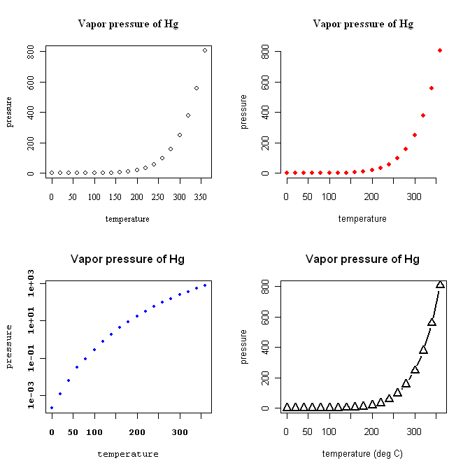
> # some really dumb examples!
> op = par(                            # store old settings in op ("old parameters")
+          mfrow=c(2,2),               # plot two rows and two cols of graphs
+          family="serif")             # use a serif font (tacky!)
> plot(pressure)                       # begin with a default plot
> title(main="Vapor pressure of Hg")   # add a main title to it
> plot(pressure,
+      bty="n",                        # no box this time
+      family="sans",                  # use a sans serif font
+      pch=16,                         # and a different data point character
+      col="red")                      # and make them red while we're at it
> title(main="Vapor pressure of Hg")   # still serif--this hasn't changed
> plot(pressure,
+      bty="o",                        # the box is back
+      family="mono",                  # use a mono spaced font
+      pch=20,                         # change the data symbols again
+      col="blue",                     # make them blue this time
+      font=2,                         # make the axis values bold
+      log="y")                        # and use a logarithmic y-axis
> title(main="Vapor pressure of Hg", family="sans")
> plot(pressure,
+      family="sans",                  # sans serif font
+      pch=2, cex=1.5,                 # new and bigger data symbols
+      type="b",                       # plot both points and lines
+      xlab="temperature (deg C)",     # customize the x-label
+      lwd=2)                          # make the plotted lines thicker
> title(main="Vapor pressure of Hg", family="sans")
> par(op)                              # reset the old graphics options

Phew! It's a lot to keep straight, isn't it? What can I say? With power comes complexity. I'm VERY far from being an expert in R graphics, so don't for a moment think the above example is all there is. We've barely scratched the surface.

Just a few more notes: You can see the color names available in R by using the colors() function. There are a whole lot (> 600) of them! Colors can also be set using hex codes, as in most graphics software. The last line of the above example resets the graphics options to their original values, IF they were saved in "op" to begin with. You can do the same thing by just closing the graphics device, as the new options only apply to the device that was opened by the "par" command.

Special Topic: Getting Big Data Labels to Fit

Try this.

> data.table = margin.table(Titanic, c(2,1))     # if you've already erased it
> dimnames(data.table) = list(
+          Sex=c("Male","Female"),
+          Class=c("First Class","Second Class","Third Class","Crew"))
> windows(4,4,12)                                # or quartz("Quartz",4,4,12) on a Mac
> barplot(data.table, beside=T, axis.lty=1)

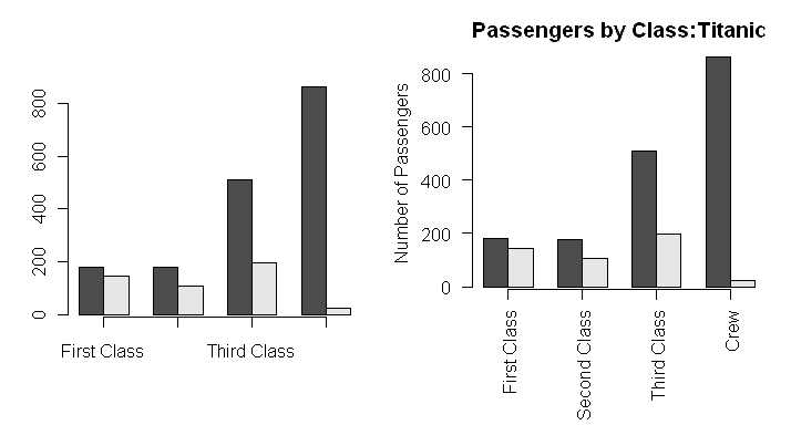
That's annoying, isn't it? The data labels on the x-axis are too long to all fit, so R has printed only those it can squeeze in (left hand graph below). A program like Excel would print those data labels vertically so they would all fit. R will as well, but it won't unless you tell it to, which in my opinion is a nice touch. It gives me control over what the graph looks like instead of having to accept whatever the software has decided. More work, but more flexibility as well.

You may have noticed in the last section the graphics option "las", which controls the orientation of axis labels. The default value is 0=always parallel to the axis, but other possibilities are 1=always horizontal, 2=always perpendicular to the axis, and 3=always vertical. Try this.

> barplot(data.table, beside=T, axis.lty=1, las=2)    # output not shown

Doesn't quite do it, does it? But don't fail to notice the value labels on the y-axis. These have now also turned perpendicular to the axis, which may be required by some editors (or instructors). This is how you would achieve it. (Note to my students: Check your APA Manual! You're going to want to know how to do this!)

We could make the font smaller, but I'm stubborn. I don't wanna! The data labels are printed in the margins of the plotting area, and we can see what those are by querying the "mar" settings.

> par("mar")
[1] 5.1 4.1 4.1 2.1

I don't know the units (and the help page does not give up this info--apparently, it is top secret), but these are respectively the bottom, left, top, and right margin sizes. What we need to do is shift the graph up in the plotting window to make room for the data labels on the x-axis.

> par(mar=c(6.4,4.1,2.7,2.1))
> barplot(data.table, beside=T, axis.lty=1, las=2)
> title(main="Passengers by Class:Titanic")
> title(ylab="Number of Passengers")

How did I know how far to shift the margins, you ask. Lots of trial and error! I also added a main title and a y-axis label just to make sure they still fit well. The x-axis doesn't really need any additional annotation.

Why not be really classy and have the x-axis labels angled at, say, 45 degrees relative to the axis? Why not, indeed! Sadly, that is one thing R will not do, at least not in the default packages.

Special Topic: Error Bars

One of the more serious shortcomings of R, in my opinion, is that it provides no convenient way to show error bars on barplots or line graphs. Error bars are such a common part of scientific graphics that I have to stand amazed at this obvious oversight. However, there is no need for despair. Adding error bars is not very difficult.

There are add-on packages that incorporate functions to do error bars. Also, various people have written scripts. For example, see Crawley (2007), page 462. However, once you understand a few simple things about R graphs, drawing your own error bars just takes a few simple steps, and you can customize them to your heart's content.

Error Bars on Barplots

Barplots are produced from a table of means (or whatever summary statistic you care to use).

> data(InsectSprays)
> names(InsectSprays)
[1] "count" "spray"
> means = with(InsectSprays, tapply(count, spray, mean))
> means
        A         B         C         D         E         F 
14.500000 15.333333  2.083333  4.916667  3.500000 16.666667
> windows(4,3,8)                            # open a graphics window; quartz("Q",4,3,8) on a Mac
> barplot(means) -> bp.out                  # default plot
> barplot(means, ylim=c(0,20), axis.lty=1)  # make room for error bars
> title(xlab="Spray")
> title(ylab="Insect Count")
> title(main="Effectiveness of Insect Sprays")

Now here's the trick to adding error bars. We need to know the x-coordinates of the centers of those bars in order to draw the error bars in the right place. And those coordinates are not 1, 2, 3, 4, 5, 6, as you might expect (as they would be for boxplots, for example). Lucky for us, we have saved those coordinates in the object "bp.out". You were wondering what that was about, weren't you?

> bp.out
     [,1]
[1,]  0.7
[2,]  1.9
[3,]  3.1
[4,]  4.3
[5,]  5.5
[6,]  6.7

Now we need a vector of errors that will determine the length of the error bars. These can be anything you want: standard errors, confidence intervals, whatever floats your boat.

> sem = function(x) sqrt(var(x)/length(x))                 # create an sem function
> errors = with(InsectSprays, tapply(count, spray, sem))
> errors
        A         B         C         D         E         F 
1.3623732 1.2329647 0.5701984 0.7225621 0.5000000 1.7936476

We could have calculated the standard errors a little more laboriously, but I've used a trick. I created a function to do it (see Writing Your Own Functions and Scripts for more about this). Now we are ready to VERY CAREFULLY add the error bars. (Once again, if you are doing all this inside a script, less care is needed as you can always make changes and redo the entire graph, but I'm living on the edge here!) We could add the error bars one at a time, but I'm going to do it with a loop. First, I'll draw some very simple error bars.

> for(i in 1:length(bp.out)) {         # repeat the following for all six bars
+    lines(x=c(bp.out[i],bp.out[i]), y=c(means[i], means[i]+errors[i]))
+ }                                    # end the loop with a curly brace

A tad bit fancier, and don't worry about redrawing the graph. We're going to draw right over the old error bars.

> for(i in 1:length(bp.out)) {
+    lines(x=c(bp.out[i],bp.out[i]), y=c(means[i]-errors[i], means[i]+errors[i]))
+ }

The loop starts with bar i=1 and draws a line connecting the points:
(bp.out[1], means[1]-errors[1]) and (bp.out[1], means[1]+errors[1]). I.e., from one standard error below the top of bar 1 to one standard error above the top of bar 1. Then it does the same for bar i=2, bar i=3, etc., until it runs out of values in bp.out.

Now we're going to get even fancier and draw error whiskers with cross bars on them. We'll do this using the arrow() function. Once again, we'll draw them right over the old error bars.

> for (i in 1:length(bp.out)) {        # repeat the following for all six bars
+    arrows(bp.out[i],means[i],bp.out[i],means[i]+errors[i],angle=90,length=.1)
+    arrows(bp.out[i],means[i],bp.out[i],means[i]-errors[i],angle=90,length=.1)
+ }                                    # curly brace ends loop

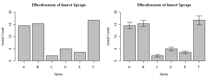And there we go!

This will be easier to remember if you know what just happened here, so let me explain. Instead of drawing each error bar individually, I used a loop, since the command for each bar is very nearly the same. To start a loop, you type for(), and inside the function you give a counter name (use i), type the word "in", then give a vector that tells how many times to execute the loop. Here, that vector amounts to 1:6, which says "execute this loop six times." Note the use of the loop counter in the arrows() function to keep track of which error bar we are drawing. The commands to be looped through are between open and close curly braces. The arrows() function draws arrows on graphs, which is to say, arrows that point to things. The syntax is different from that of lines() in so far as the way the xy-coordinates are given:

arrows(x0, y0, x1, y1, angle= length= )

The first two values, x0 and y0, are the starting coordinates of the arrow. We started them at the center of a bar and the mean. The next two values are the ending coordinates of the pointy end of the arrow. We ended them at the center of a bar, and the mean ± error. The "angle=" option gives the angle of the arrowhead to the shaft--90° in this case, or at right angles. The "length=" option gives the length of each side of the arrowhead. Frankly, I'm a bit surprised they came out so long in this example, but once again, if you are scripting this, you can change them until they agree with your own artistic sense. One more thing you should not fail to notice--the first and second line of that loop differ by only one character. So don't retype the entire line just to change one little thing. Use the up arrow key to recall the previous line and edit it.

Error Bars on Line Graphs

Error bars on line graphs are even easier. Nevertheless, I am going to do the sensible thing and script this one in the script editing window (see Writing Your Own Functions and Scripts) so I can get it just the way I want it.

> ls()
[1] "bp.out"       "errors"       "i"            "InsectSprays" "means"       
[6] "sem"         
> rm(bp.out,errors,i,InsectSprays,means)    # save that sem function
> graphics.off()                            # close any old graphics windows
> data(Orange)
> names(Orange)
[1] "Tree"          "age"           "circumference"
> means = with(Orange, tapply(circumference, age, mean))
> errors = with(Orange, tapply(circumference, age, sem))

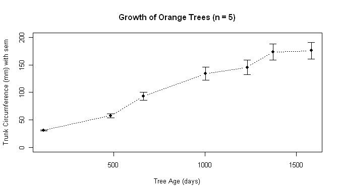
The data give information on the growth of five orange trees, specifically trunk circumference in millimeters at seven ages in days ranging from 118 to 1582. Since the explanatory variable is numeric, a line graph would be more appropriate than a bar graph.

> age.days = Orange$age[Orange$Tree==1]     # get one copy of x-coords
> rm(Orange)                                # don't need this anymore
> plot(age.days,means,type="b")             # let's see what we've got
> errors
       118        484        664       1004       1231       1372       1582 
 0.6324555  3.6523965  7.7097341 11.5991379 13.0713427 14.6853669 14.8842198

Okay, close that old graphics window, and then open a new one.

> graphics.off()
> windows(7,4,10)                 # quartz("Q",7,4,10) on a Mac

Now I'll shift over to a script...

### Begin copying here.
plot(age.days, means,
     type="b", pch=16, lty=3, ylim=c(0,200),
     ylab="Trunk Circumference (mm) with sem",
     xlab="Tree Age (days)",
     main="Growth of Orange Trees (n = 5)")
len = .07
for (i in 1:7) {
     arrows(age.days[i], means[i],
            age.days[i], means[i]+errors[i],
            angle=90, length=len)
     arrows(age.days[i], means[i],
            age.days[i], means[i]-errors[i],
            angle=90, length=len)
}
### End copying here.

You can copy and paste this script into the R script editor and play with it all you want.

A note: Yes, it is possible to draw a custom x-axis with tick marks and value labels that correspond to the values of age.days in the data. I'd have to look it up, so you do, too!

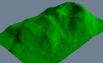
I admit, compared to having a proper error bars function in R, this is a pain in the anatomy. However, once you've done it a few times, it's very quick, and it's a small price to pay for the power of the R graphics engine. Let's see Excel draw a volcano!

Splitting the Graphics Window Into Multiple Plotting Areas

There are two ways to do this, both with advantages and disadvantages. In my opinion, which I'll be sure to give you, one way is clearly superior.

One way is to use the split.screen() function. As it's main argument, this function takes a two-element vector telling how may rows and columns of plotting areas you want in the graphics window. The plotting areas are numbered across the rows. Use screen(n=) to specify the active plotting area. The help screen says you can use erase.screen(n=) to erase one of the plottiing areas, but this doesn't work on my Mac. Here is an example, which I will give without command prompts so that you can copy and paste it. It illustrates a few of the finer points of using this method.

graphics.off()                         # turn off any old plots
split.screen(c(2,2))                   # two rows of two graphs each
# output is [1] 1 2 3 4
screen(n=1)                            # upper left plotting area
plot(eruptions ~ waiting, data=faithful, cex=.5)
title(main="Old Faithful Data")        # screen 1 still active
screen(n=4)                            # switch to the lower right area
hist(faithful$eruptions, prob=T, main="")
lines(density(faithful$eruptions))
screen(n=3)                            # switch to the lower left area
acf(faithful$eruptions, main="")
title("Autocorrelation: Eruptions")
screen(n=4)                            # forgot something!
title(main="Kernel Density: Eruptions")
screen(n=2)                            # switch to upper right
plot(faithful$eruptions[1:50], pch=16, cex=.3, type="b", ylab="Eruption Time (min)")
title(main="Serial Plot: Eruptions")

As you can see, you can jump willy nilly from plotting area to plotting area, and even go back to one if you forgot something. The next function, par(mfrow=c(2,2)), is not so flexible but, in my opinion, produces a superior result. With this function, plotting must progress across the rows of the plotting areas, and there is no going back. (Note: A related function, par(mfcol=c(2,2)), works the same except that plotting progresses down the columns. The vector still gives the number of rows followed by the number of columns of plotting areas desired.)

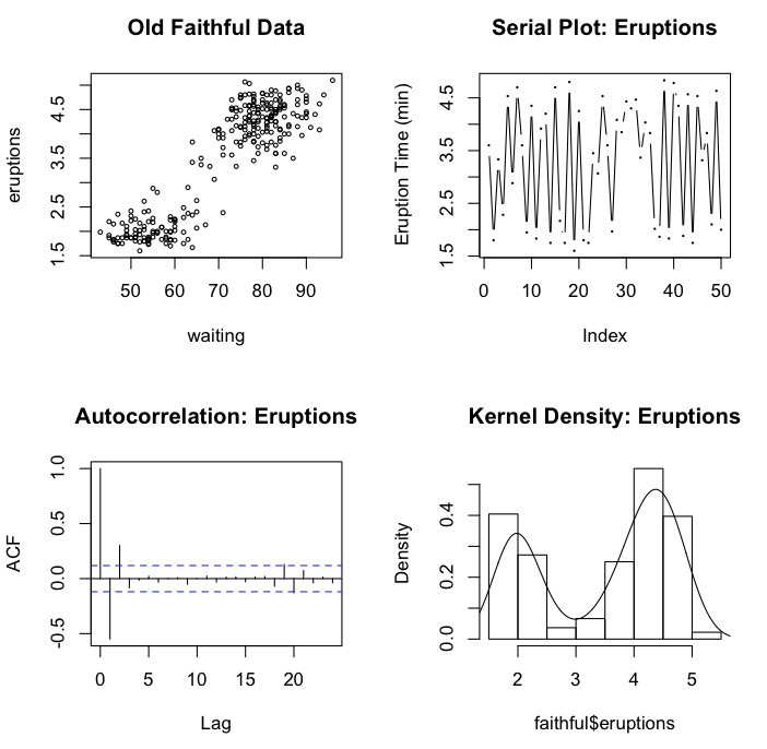
graphics.off()
par(mfrow=c(2,2))                      # two rows of two graphs each
# upper left plotting area is first no matter what!
plot(eruptions ~ waiting, data=faithful, cex=.5)
title(main="Old Faithful Data")        # low level function so no change in plotting area
# upper right plotting area comes next, the switch caused by using a high level function
plot(faithful$eruptions[1:50], pch=16, cex=.3, type="b", ylab="Eruption Time (min)")
title(main="Serial Plot: Eruptions")
# then lower left area
acf(faithful$eruptions, main="")
title("Autocorrelation: Eruptions")    # don't forget, because there's no going back!
# and finally the lower right area
hist(faithful$eruptions, prob=T, main="")
lines(density(faithful$eruptions))
title(main="Kernel Density: Eruptions")
# a new high level function here would start cycling through the plotting areas again

Compare to the previous graph. I suppose they could be made to look identical with enough fiddling with graphics parameters. Another advantage of the first method is that plotting areas can be further subdivided (so they tell me--I've never done it), so take your pick.

revised 2016 February 1