SIMPLE PATH ANALYSIS

Preliminaries

Once again, I will begin with the warning that I am not an expert in path analysis. I know some of the basics, so you should take the word "simple" in the title of this tutorial very seriously. I think you would be well served, if you are not familiar with these topics, to read the Hierarchical Regression and Simple Mediation Analysis tutorials first. In fact, this tutorial might be seen as an extension of the one on mediation. And since all of these techniques are simple extensions of Multiple Regression, it might be useful to be familiar with those techniques as well. (Might? Did he really say might?)

There are R packages for path analysis. A good one is the "lavaan" package (stands for latent variable analysis). I won't be using that package here, but there is a good YouTube video on it. The lavaan manual can be found at CRAN. There are also some tutorials located here.

At the end of this tutorial, I will demonstrate the use of the "sem" package for relatively simple path analysis.

What Can You Tell From a Correlation Coefficient?

If two variables are correlated, then you know that certain values of one tend to go with certain values of the other. A positive Pearson's r, for example, between variables A and B means that larger values of A tend to go with larger values of B, and smaller values with smaller values. The closer the r value is to +1 (or -1 in the case of a negative correlation), the stronger that tendency is. On the other hand, as the r value gets closer to zero, the relationship gets weaker and weaker. Everybody who's taken STAT 101 knows that much. But why? Why are A and B correlated?

There are basically four possibilities. 1) The correlation is spurious. That is, there is no connection between A and B and the correlation between them is entirely coincidental. 2) A causes B, or B causes A. We can't really say which from the fact of a simple correlation. 3) A may not directly cause B, or vice versa, but the effect of A on B, or B on A, may be mediated by one or more intervening variables. 4) A and B may have a common cause, which may also be mediated by intervening variables. The following diagram illustrates these possibilities. The arrows in this diagram represent cause and effect relationships. More complex possibilities exist, but you get the idea, I'm sure.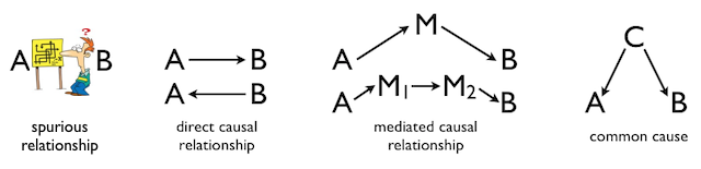

The elements of this diagram form the bits and pieces of a path analysis.

Three things are necessary to show a cause and effect relationship between two variables. 1) There must be concomitant variation, or covariation. When A changes, B must also change. This is basically the information we get from the correlation coefficient, and it's about all we get from a correlation coefficient. So a correlation alone is not sufficient to show cause and effect, although we might argue that it's necessary to show cause and effect. 2) There must be sequential ordering. That is, causes must happen before their effects. If A causes B, then A has to occur before B. 3) Rival explanations, such as a common cause for example, must be eliminated.

In path analysis, we are going to attempt to draw a diagram that shows how several, possibly correlated, variables are related. That diagram will be called a path diagram. The important thing to remember is, the path diagram comes FIRST. Path analysis is a way of finding confirmatory, or supporting, evidence from correlational data for a causal theory that we already have. The causal theory does not come from the path analysis; it precedes the path analysis. The path analysis simply attempts to find correlational evidence that is consistent with the pre-existing causal theory. So the hard thinking has to be done first.

For example, suppose we have a theory about what leads to success in studying science. We might summarize that theory with the following path diagram.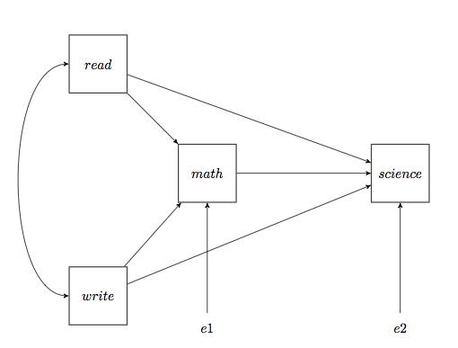

The diagram proposes that success at science is a function of three things (in addition to some other, unknown or unspecified, inputs). First is math. If you can't do math, you're dead in the water as far as success at science is concerned. In addition, there is also a direct causal relationship with reading ability and with writing ability. But in addition to this direct relationship between reading and science (and writing and science), there is also an indirect or mediated relationship. Reading is also important to your ability to do math. (Gotta be able to read those word problems!) So part of the effect of reading on science is direct, and part is indirect or mediated. The same goes for writing ability. Reading and writing ability are also correlated, as shown by the curved arrow with double arrowheads, but that's basically additional information not directly relevant to the cause of success at science. The path analysis will now attempt to find evidence consistent with this theory. It will NOT PROVE the theory, but it will be consistent with this path diagram we've drawn, or so we hope. (By the way, the above diagram is not mine. I snitched it from the website of the UCLA Institute for Digital Research and Education.)

A few notes: First of all, notice that there are no reciprocal paths in this diagram. That is, the causality arrows always point unambiguously in one direction only. There are no "feedback loops," either direct or indirect. Reciprocal paths are certainly possible, in real life as well as in path analysis, but not in "simple" path analysis. Second, all of these variables are at least interval scale variables. If we had any ordinal or nominal scale variables here, we'd be stumped. I'm not saying it isn't possible to do the analysis with those sorts of variables, but it isn't "simple." Third, could we draw any more arrows in this diagram if we wanted to? Not if we want to follow the rule of no two-way paths and no loops (and we do want to follow that rule). We could draw a causal (straight-arrow) path from read to write or write to read, I suppose, but we already have that curved correlational arrow, which is handling the correlation there. So the answer is no. Therefore, this model is said to be a saturated model. All possible paths are present. Notice I didn't say it is the saturated model. It is a saturated model. Others are possible.

The Path Analysis

The function of path analysis is to tell us, first, if all those pathways exist, and second, how strong they are. The data for the analysis are at the UCLA website I linked to above and can be read directly into R as follows.

> ucla = read.table("http://www.ats.ucla.edu/stat/data/hsb2.txt", header=T, row.names=1)
> dim(ucla)
[1] 200  10
> summary(ucla)
     female           race           ses            schtyp    
 Min.   :0.000   Min.   :1.00   Min.   :1.000   Min.   :1.00  
 1st Qu.:0.000   1st Qu.:3.00   1st Qu.:2.000   1st Qu.:1.00  
 Median :1.000   Median :4.00   Median :2.000   Median :1.00  
 Mean   :0.545   Mean   :3.43   Mean   :2.055   Mean   :1.16  
 3rd Qu.:1.000   3rd Qu.:4.00   3rd Qu.:3.000   3rd Qu.:1.00  
 Max.   :1.000   Max.   :4.00   Max.   :3.000   Max.   :2.00  
      prog            read           write            math      
 Min.   :1.000   Min.   :28.00   Min.   :31.00   Min.   :33.00  
 1st Qu.:2.000   1st Qu.:44.00   1st Qu.:45.75   1st Qu.:45.00  
 Median :2.000   Median :50.00   Median :54.00   Median :52.00  
 Mean   :2.025   Mean   :52.23   Mean   :52.77   Mean   :52.65  
 3rd Qu.:2.250   3rd Qu.:60.00   3rd Qu.:60.00   3rd Qu.:59.00  
 Max.   :3.000   Max.   :76.00   Max.   :67.00   Max.   :75.00  
    science          socst      
 Min.   :26.00   Min.   :26.00  
 1st Qu.:44.00   1st Qu.:46.00  
 Median :53.00   Median :52.00  
 Mean   :51.85   Mean   :52.41  
 3rd Qu.:58.00   3rd Qu.:61.00  
 Max.   :74.00   Max.   :71.00

There's some interesting stuff here, but the columns we need are columns 6, 7, 8, and 9, so I'm going to grab those columns and throw the rest of them away. Well, on second thought, maybe I'll keep column 10 as well. Could be interesting. Then we'll look at a correlation matrix.

> ucla = ucla[,6:10]
> cor(ucla)
             read     write      math   science     socst
read    1.0000000 0.5967765 0.6622801 0.6301579 0.6214843
write   0.5967765 1.0000000 0.6174493 0.5704416 0.6047932
math    0.6622801 0.6174493 1.0000000 0.6307332 0.5444803
science 0.6301579 0.5704416 0.6307332 1.0000000 0.4651060
socst   0.6214843 0.6047932 0.5444803 0.4651060 1.0000000

> uclast = scale(ucla)            # create a matrix of standardized variables
> uclast = as.data.frame(uclast)  # convert matrix to data frame

• science - from math, read, and write (and error, which is not "causal" or causes unknown)
• math - from read and write (and error)

> summary(lm(science ~ math + read + write, data=uclast))  # some output has been deleted

Coefficients:
              Estimate Std. Error t value Pr(>|t|)    
(Intercept) -2.027e-16  5.038e-02   0.000  1.00000    
math         3.019e-01  7.255e-02   4.161 4.75e-05 ***
read         3.123e-01  7.112e-02   4.390 1.85e-05 ***
write        1.977e-01  6.775e-02   2.918  0.00393 ** 
---
Residual standard error: 0.7125 on 196 degrees of freedom
Multiple R-squared:  0.4999,	Adjusted R-squared:  0.4923 
F-statistic: 65.32 on 3 and 196 DF,  p-value: < 2.2e-16

> summary(lm(math ~ read + write, data=uclast))            # some output has been deleted

Coefficients:
              Estimate Std. Error t value Pr(>|t|)    
(Intercept) -5.831e-16  4.948e-02   0.000        1    
read         4.563e-01  6.182e-02   7.382 4.29e-12 ***
write        3.451e-01  6.182e-02   5.583 7.76e-08 ***
---
Residual standard error: 0.6997 on 197 degrees of freedom
Multiple R-squared:  0.5153,	Adjusted R-squared:  0.5104 
F-statistic: 104.7 on 2 and 197 DF,  p-value: < 2.2e-16

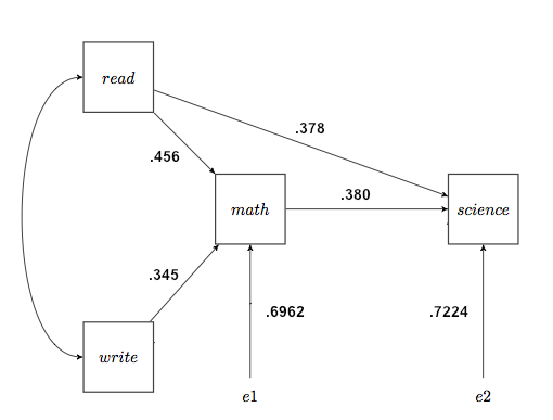
Fourth, we write the appropriate regression coefficients, which are now called the path coefficients, on the path diagram. The error inputs, if you want them, are from the R-squared values, and specifically are sqrt(1−R-squared). I'll show those calculations on the diagram, which is not customary. The error inputs represent not only random error but also possibly other variables not included in the model that may have causal input into a given box. The diagram that results is called the output path diagram. I have also written the correlation between read and write, .597, along the curved arrow, although technically we could say that's not part of the path model. Nevertheless, we will use it below. Such curved, correlational arrows should be drawn only between exogenous variables.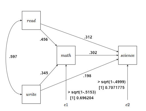

Finally, we use the output diagram to assess our theory. Are all of these paths present, or should some be deleted? It appears that our path analysis is consistent with our theory. The theory is supported by the data, but certainly by no means proven.

Now I would urge you to repeat this analysis, but with socst (social studies, I assume) in place of science. Testing for the significance of path coefficients may be as simple as looking at the test on the corresponding regression coefficients in the regression analyses, or it may be considerably more complex than that, depending up what source you read, but it appears to me that the middle of the diagram, the math part, drops out when the end variable is socst (which could explain why we in psychology get a lot of our majors as refugees from the hard sciences--most psychology majors can't do math, in my experience). The coefficient from math to social studies becomes .108, which is weak at best and nonsignificant in the regression analysis. At the same time, the coefficient from write to social studies becomes .326, indicating a much stronger influence of writing ability on social studies success than on science success. And you don't have to read a lot of published scientific papers to get that!

Direct, Indirect, and Total Effects

Let's look at the effect of read on science. The effect "travels" through two pathways, one direct and one indirect. The direct path has a strength of .312, which is the beta coefficient from the regression of science on math, read, and write. As a path coefficient, we interpret it the same way. The direct effect of read on science is .312 standard deviations, which is to say, a 1 SD change in read creates a .312 SD change in science. (These are scores on achievement tests.)

There is also an indirect effect of read on science, which is mediated by math. The strength of this effect is the product of all the path coefficients along that path, i.e., .456*.302=.138. The strength of this effect is interpreted the same way.

That suggests that the total effect of read on science, at least in our model, should be the sum of those two things. I'm going to do more than suggest it, I'm going to say it! The total effect of read on science is .312+.138=.450, and it also has the same interpretation: a 1 SD change in read produces a total change in science of .450 SD. Some of that change occurs directly, but some is mediated via math.

Using this simple method, we can create a table of how each of three "causes" has an "effect" on science. (Note: To calculate direct and indirect effects, you cannot follow curved paths, and you must follow the causal arrows in the direction they are pointing.)

It's an intereesting table, isn't it? It suggests that, of the three causes in our model, it's read that has the greatest total effect, while write and math have equal total effects, something we wouldn't have gotten from the regression analysis, which just shows direct effects. The catch there is the phrase "in our model." If our model contained different or additional variables, we might be getting different results. The investigation, as they say, is ongoing. No path analysis will ever give us the final answer. ("All models are wrong, but some are useful" - George Box. "The map is not the territory" - Alfred Korzybski.)

Decomposition of Correlations

Why do the correlations among these variables have the values that they do? The path model can be used to "explain" the correlations, sort of. If you don't place too much emphasis on the word "explain" while reading that sentence. The path model can be derived from the correlation matrix, and now we are going to use to the path model to explain the correlation matrix. One might be tempted to use words such as "tautological" or "circular" to describe what we are about to do. Nevertheless, it's a useful exercise, as we'll see.

First, we need to know Wright's rules of tracing. If you think of the path model as a diagram of sidewalks between buildings on a campus, we ask, "How many ways are there to walk from read to science?" The catch is, we have to follow these rules:

• No loops are allowed. We can't pass through the same variable (building) twice.
• Although we're allowed to walk backwards along an arrow, i.e., in the direction opposite of which the arrow is pointing, we can't go forwards and then backwards. This is the same thing as saying we can't enter a box and leave a box through an arrowhead. For example, in our model, we can't go from read to math to write.
• Only one curved arrow is allowed in any route.

Thus, to get from read to science, we could take these routes. I'll calculate the effects as we walk the routes.

• Read to science directly. Effect = .312.
• Read to math to science. Effect = .456*.302=.138.
• Read to write to science. Effect = .597*.198=.118.
• Read to write to math to science. Effect = .597*.345*.302=.062

Now we'll add up the effects along all those possible routes.

.312 + .138 + .118 + .062 = .630

Compare this value to the correlation between read and science. I'll let you do write to science. Hint: It's the total effect of write plus the read-write correlation times the total effect of read. The tough one is math and science.

• Math to science directly. Effect = .302.
• Math to read to science. Effect = .456*.312=.142.
• Math to read to write to science. Effect = .456*.597*.198=.054.
• Math to write to science. Effect = .345*.198=.068.
• Math to write to read to science. Effect = .345*.597*.312=.064.

The sum is:

.302 + .142 + .054 + .068 + .064 = .630

Which is amazingly close to correct considering the amount of rounding error we were accumulating.

This reproduction of the correlation matrix from the output path diagram will work only if the model was calculated from standardized variables and only if the path model is saturated. If we delete one or more of the arrows in the above path model, the correlations will be off. This serves as one basis for testing the goodness of fit of a path model. Using our model, how close can we come to reproducing the correlation matrix (or variance-covariance matrix)? A saturated model will always fit the data perfectly and, therefore, really doesn't teach us very much. We begin learning things when we start deleting paths without doing too much damage to our ability to reproduce the correlation matrix.

The statistic derived from this method is called the chi-square goodness of fit statistic (although it is really a "badness-of-fit" statistic). There is a whole alphabet soup of other fit statistics derived from this chi-square value, but they are beyond the scope of this tutorial, and I will refer you to another source, such as Schumacker and Lomax (2010), or the documentation for your path analysis software. (A good summary is available here.)

Sample Size

Path analysis is definitely a large sample technique. The following guidelines are often given. Sample sizes of less than 100 are considered small and might call into question the accuracy of a path analysis. Sample sizes between 100 and 200 are adequate. Sample sizes greater than 200 are considered large and are to be preferred.

The ratio of cases to parameters, i.e., subjects to path coefficients being estimated should be 20:1 or larger, although 10:1 is considered "okay" in a pinch.

Finally, the maximum number of paths that should exist in the model is purely a matter of mathematical expediency, and is v(v+1)/2, where v is the number of variables (boxes) in the model.

Path Analysis and Mediation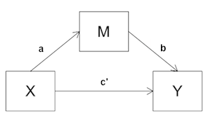

You have surely noticed the similarities between path modeling and Mediation Analysis. The path diagram for a simple mediation analysis is shown at right. The model shows a direct effect of X on Y, and an indirect or mediated effect of X on Y. The question we asked in mediation analysis was, when the mediated path is included in the model, how much is left for the direct path to explain? If the path coefficient on X->Y goes to zero, or becomes nonsignificant, then we have complete mediation. If it decreases but does not go to zero, then we have partial mediation. If it stays the same as it was without the mediated path, or not significantly different from that, then we have no mediation.

If you look at the bottom three boxes (write, math, science) in the path diagram above, you'll see what amounts to a mediation analysis. The relationship of write to science is substantial (r=.57). Is that all direct? Or is some or perhaps even all of it due to needing to be able to write to do math? (They are not entirely dissimilar skills. They both involve logical interpretation and manipulation of symbolic relationships, and that skill is normally acquired first in reading and writing.)

In the Baron and Kenny approach to mediation analysis (see that tutorial), the analysis would follow a four-step procedure. First through third, we have to show that all of the paths in the diagram are significant. This can be done either by calculating correlations, or by looking at simple regression coefficients, and checking for statistical significance.

> summary(lm(science ~ write, data=ucla))$coef
              Estimate Std. Error  t value     Pr(>|t|)
(Intercept) 20.4036552 3.26895123 6.241652 2.582425e-09
write        0.5958568 0.06097055 9.772863 1.168988e-18
> summary(lm(science ~ math, data=ucla))$coef
            Estimate Std. Error   t value     Pr(>|t|)
(Intercept) 16.75789 3.11622943  5.377619 2.114967e-07
math         0.66658 0.05828216 11.437119 1.388621e-23
> summary(lm(math ~ write, data=ucla))$coef
              Estimate Std. Error   t value     Pr(>|t|)
(Intercept) 20.4377529 2.96237257  6.899116 6.892839e-11
write        0.6102747 0.05525243 11.045211 2.086665e-22

> summary(lm(science ~ math + write, data=ucla))$coef
              Estimate Std. Error  t value     Pr(>|t|)
(Intercept) 10.6813845 3.29339118 3.243278 1.387921e-03
math         0.4757015 0.07094004 6.705685 2.068155e-10
write        0.3055482 0.07011573 4.357770 2.113555e-05

The significance test for the mediation model that was used in the mediation tutorial was the one based on the normal model, namely, Sobel's z. Let's run that now using the mediate() function from the tutdata folder (if you have it--if not, you can get it here).

> source("tutdata/mediate.R")     # assuming this is in your working directory
> with(ucla, mediate(x=write, y=science, m=math))
       a        b        c       cp  sobel.z        p 
0.610275 0.475702 0.595857 0.305548 5.714924 0.000000

"Whoa! Back the truck up here a minute! What do you mean the significance test 'was the one based on the normal model?' Are you saying there are others?" Couldn't slip that by ya, huh? MacKinnon, et al. (2002), using a simulation method, checked the normal model test for Type I and Type II error rates and statistical power. They compared it to--take a deep breath--thirteen other methods for testing mediation and intervening variable effects.

Sobel's z is a test of the indirect effect of X on Y, i.e., the effect through the mediator. It tests this effect by calculating the indirect effect by multiplying the path coefficients, a*b, and then dividing that by its standard error. In simple mediation, it turns out this is equivalent to testing the difference between the X->Y path coefficients without and with M in the model. The problem with this method is that it assumes a*b is normally distributed, which it often is not (or so I'm told). MacKinnon, et al., also showed that the method, including the four-step verification of the paths, has low statistical power.

Mallinckrodt, et al. (2006), summarized a bootstrap method for assessing the significance of an indirect (mediated) effect based on a method proposed by Shrout and Bolger (2002). They provided scripts for doing the test in six software packages, none of which was R. The steps they followed were (p. 374):

• "Using the original data set of N cases as a population reservoir, create a bootstrap sample of N cases by random sampling with replacement."
• "Calculate a, b, and a * b based on this bootstrap sample, and save the results to a file."
• "Repeat Steps 1 and 2 a total of J times."
• "Examine the distribution of J estimates, and if alpha < .05, determine the 2.5 and 97.5 percentile values of a * b."

This sounds like it ought to be a piece of cake in R. (And would have been if the assign() function had worked in a reasonable way, which apparently it doesn't!) Here is a script. Copy and paste it into a script window (File > New Script in Windows; File > New Document on a Mac), tell it what your data frame is and what columns you want as X, Y, and M in that order, and set J if you want something other than 1000 iterations. Then execute the script.

### begin copying here
Data = ucla[,c(2,4,3)]       # be sure this is in X, Y, M order
J = 1000                     # set this to number of iterations desired
### don't change anything below this line ###
colnames(Data) = c("X","Y","M")
N = dim(Data)[1]
results = numeric(J)
for(i in 1:J) {
    Cases = sample(1:N, N, replace=T)
    tempdf = Data[Cases,]
    a = coef(lm(M ~ X, tempdf))[2]
    b = coef(lm(Y ~ M + X, tempdf))[2]
    results[i] = a * b
}
summary(results)
quantile(results, c(.025,.975))
### end copying here and paste into a script window

> summary(results)
   Min. 1st Qu.  Median    Mean 3rd Qu.    Max. 
 0.1224  0.2549  0.2903  0.2900  0.3234  0.4495 
> quantile(results, c(.025,.975))
     2.5%     97.5% 
0.1914613 0.3869541

(Further note: Here's another question I have. I've been warned in various sources NOT to standardize the variables in a mediation analysis. But these scores are from achievement tests. They are already standardized, but on a T-scale rather than a z-scale. What could it possibly hurt if I rescaled them to z-scores? It's a linear transformation, like changing inches to centimeters. If that would affect the outcome of a statistical analysis, then I would have to consider that analysis highly suspect!)

Mallinckrodt, et al., reported that this method is a statistically powerful alternative to the Sobel method, especially for small effects and smaller sample sizes. They recommended using a bias-corrected bootstrap confidence interval. This can be obtained with the boot() function in the "boot" library. I recommend you read the Resampling Methods tutorial before venturing into these murky waters, because the boot() function and its helper cousin boot.ci() are very obtuse and tricky. For the record, here's how you would do it.

> library("boot")                      # load the boot library
> ab = function(data, i) {
+    a = coef(lm(math ~ write, data[i,]))[2]
+    b = coef(lm(science ~ math + write, data[i,]))[2]
+    a * b
+ }                                    # write a function for the statistic to be bootstrapped
> boot.out = boot(data=ucla, statistic=ab, R=1000)
> boot.out

ORDINARY NONPARAMETRIC BOOTSTRAP

Call:
boot(data = ucla, statistic = ab, R = 1000)

Bootstrap Statistics :
     original       bias    std. error
t1* 0.2903086 0.0001339031  0.05116755

> quantile(boot.out$t, c(.025,.975))
     2.5%     97.5% 
0.1963277 0.3946157

> boot.ci(boot.out, type="bca")
BOOTSTRAP CONFIDENCE INTERVAL CALCULATIONS
Based on 1000 bootstrap replicates

CALL : 
boot.ci(boot.out = boot.out, type = "bca")

Intervals : 
Level       BCa          
95%   ( 0.1958,  0.3942 )  
Calculations and Intervals on Original Scale

> boot.ci(boot.out, type="perc")
BOOTSTRAP CONFIDENCE INTERVAL CALCULATIONS
Based on 1000 bootstrap replicates

CALL : 
boot.ci(boot.out = boot.out, type = "perc")

Intervals : 
Level     Percentile     
95%   ( 0.1962,  0.3950 )  
Calculations and Intervals on Original Scale

MacKinnon, et al., recommended the "test of joint significance" (TJS) as the best overall test of the mediation effect. All that involves is looking at the X->M path and the M->Y path and seeing that they both have significant regression coefficients. Frankly, I don't see how this answers some of the questions I laid out above, but, okay! In a later study, MacKinnon found from Monte Carlo simulation that the bootstrap method is subject to inflated Type I error rates when one of the two component paths of the mediation effect is zero in the population but not zero in sample due to sampling error, and the other path is substantially greater than zero. Perhaps a reasonable suggestion here would be to examine the significance of the two paths first, a la the TJS method, and then use bootstrap to get a reasonable interval estimate of the size of the indirect effect. Mallinckrodt, et al., came to a similar conclusion.

Which brings me to, hopefully, the final point I want to make about mediation analysis. James, Muliak, and Brett (2006) wrote, "The primary problem with tests for mediation evolves from the fact that different statistical strategies are available" (p. 233). Now there's a statement that certainly stands on its own, doesn't it?! I would imagine, if you can't figure out how it should be done, that could be a problem!

James, et al., compared two approaches to mediation analysis, which they called the Baron and Kenny, or B-K, approach, which is the one outlined above and in the Mediation Analysis tutorial, and the structural equation modeling, or SEM, approach (of which path analysis is a simple version). The SEM people argue that the most parsimonious mediation model is the complete mediation model, which is depicted in the following diagram (from James, et al., Figure 1).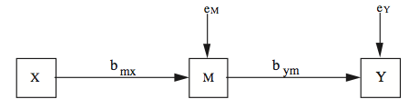

This model contains two endogenous variables, M and Y, and, therefore, requires two least squares estimating equations, one estimating the path coefficient on the X->M path, and another estimating the path coefficient on the M->Y path. In this model, the direct X->Y path is set theoretically to 0. For the model to be supported, both b_mx and b_ym must be significant. So far, we have the TJS method of testing mediation advocated by MacKinnon, et al. This is clearly not sufficient to show complete mediation, however. But if complete mediation exists, then the correlation between X and Y, r_xy, should be accounted for by the mediated route in the path diagram. That is, it should be true that r_xy = b_mxb_ym. (NOTE: Only if standardized path coefficients are used.)

Referring to the mediation diagram at the top of this section, we see that we have a saturated path model. Therefore, it should be true that r_xy = ab + c'. Thus, if c' = 0, then the above condition will hold. How do we test this? I've been unable to find anyone who's willing to commit to a specific test. (But see the next section.) For the complete mediation model, the relevant values of b_mx and b_ym would be...

> coef(lm(math ~ write, data=uclast))
  (Intercept)         write 
-4.803797e-16  6.174493e-01 
> coef(lm(science ~ math, data=uclast))
 (Intercept)         math 
5.131579e-17 6.307332e-01

> 6.174493e-01 * 6.307332e-01
[1] 0.3894458

> cor.test(uclast$write, uclast$science)$conf.int
[1] 0.4688034 0.6571717

> file = "http://ww2.coastal.edu/kingw/statistics/R-tutorials/text/loneliness.csv"
> lone = read.csv(file)      # it's also in the tutdata folder
> dim(lone)
[1] 112   5
> lonest = scale(lone)
> lonest = as.data.frame(lonest)
> cor(lonest)                # standardization does not change the correlations
          embarrass   emotiso socialiso
embarrass 1.0000000 0.2875657 0.4173950
emotiso   0.2875657 1.0000000 0.6397209
socialiso 0.4173950 0.6397209 1.0000000

> coef(lm(socialiso ~ embarrass, data=lonest))
  (Intercept)     embarrass 
-2.570672e-16  4.173950e-01 
> coef(lm(emotiso ~ socialiso, data=lonest))
 (Intercept)    socialiso 
6.711069e-17 6.397209e-01 
> 4.173950e-01 * 6.397209e-01
[1] 0.2670163

> cor.test(lonest$embarrass, lonest$emotiso, data=lonest, conf.level=.9)$conf.int
[1] 0.1374858 0.4247380

Deleting Paths from a Path Model

Let's go back to the full path model of trying to explain science success from reading, writing, and math. The output path diagram is back there quite a ways, so I'll reproduce it here.

All of these path coefficients were significant in the regression analyses. The "least significant" one was write->science, with p=.004. Let's say we're having some sort of theoretical difficulty with that path, and we want to see what happens when we delete it. Would deleting the path significantly reduce the goodness of fit of our model? We can find out by calculating a fit index called Q, which Schumacker and Lomax refer to as a "traditional non-SEM path model-fit index."

We begin by calculating the generalized squared multiple correlation. We do this as follows.

R_m² = 1 - e1²e2²e3²...

There is an e for each endogenous variable. In our model we have two of those, so...

R_m² = 1 - .6962²*.7072² = .7576

Now we calculate the reduced path model, i.e., dropping the write->science path, and from that we do the same calculation.

> summary(lm(science~math+read,uclast))     # some output deleted
Coefficients:
              Estimate Std. Error t value Pr(>|t|)    
(Intercept) -1.644e-16  5.134e-02   0.000        1    
math         3.801e-01  6.869e-02   5.534 9.90e-08 ***
read         3.784e-01  6.869e-02   5.509 1.12e-07 ***
---
Residual standard error: 0.726 on 197 degrees of freedom
Multiple R-squared:  0.4782,	Adjusted R-squared:  0.4729 
F-statistic: 90.27 on 2 and 197 DF,  p-value: < 2.2e-16

> sqrt(1-.4782)
[1] 0.7223573

> summary(lm(math~write+read,uclast))       # some output deleted
Coefficients:
              Estimate Std. Error t value Pr(>|t|)    
(Intercept) -5.831e-16  4.948e-02   0.000        1    
write        3.451e-01  6.182e-02   5.583 7.76e-08 ***
read         4.563e-01  6.182e-02   7.382 4.29e-12 ***
---
Residual standard error: 0.6997 on 197 degrees of freedom
Multiple R-squared:  0.5153,	Adjusted R-squared:  0.5104 
F-statistic: 104.7 on 2 and 197 DF,  p-value: < 2.2e-16

> sqrt(1-.5153)    # Nothing has changed in this part of the model. Why?
[1] 0.696204

And the new value of the generalized squared multiple correlation is...

R_n² = 1 - .6962²*.7224² = .7471

Finally, Q is the ratio of those two values subtracted from 1.

Q = (1 - R_m²) / (1 - R_n²)
= (1 - .7576) / (1 - .7471)
= .9585

Q will always be a number between 0 and 1, and the closer it is to 1, the less damage we've done to our model fit by dropping the path. A significance test on Q is provided by the following formula.

W = -(N - d) log_eQ

N is the sample size for the path model, and d is the number of paths we've dropped from the model. (Note: It is always best when simplifying a model to do so by dropping one path at a time.)

W = -(200 - 1) * log(.9585) = 8.435

W is distributed approximately as chi-squared with d degrees of freedom.

> pchisq(8.435, df=1, lower=F)
[1] 0.003680669

Using the sem Package for Path Analysis

A relatively simple interface to path analysis is provided by the "sem" package, created by John Fox, and authored by Fox, Nie, and Byrnes. Here is a link to the package documentation at CRAN. The first thing we have to do is install the package, since it is not part of the default download. (See the Package Management tutorial for details on installing optional packages.)

> install.packages("sem")    # output not shown
> library("sem")             # must be loaded before we can use it

R.sci <- readMoments(names=c("read","write","math","science"))
1
0.5967765 1
0.6622801 0.6174493 1
0.6301579 0.5704416 0.6307332 1

mod.sci <- specifyModel()
read -> math, gam31
write -> math, gam32
read -> science, gam41
write -> science, gam42
math -> science, beta43
math <-> math, phi33
science <-> science, phi44

sem.out <- sem(mod.sci, R.sci, N=200, fixed.x=c("read","write"))

> effects(sem.out)

 Total Effects (column on row)
             read     write      math
math    0.4563133 0.3451323 0.0000000
science 0.4499934 0.3018961 0.3018541

 Direct Effects
             read     write      math
math    0.4563133 0.3451323 0.0000000
science 0.3122534 0.1977165 0.3018541

 Indirect Effects
           read     write math
math    0.00000 0.0000000    0
science 0.13774 0.1041796    0

> summary(sem.out)

 Model Chisquare =  0   Df =  0 Pr(>Chisq) = NA
 AIC =  14
 BIC =  0

 Normalized Residuals
     Min.   1st Qu.    Median      Mean   3rd Qu.      Max. 
0.000e+00 0.000e+00 1.216e-15 9.855e-16 1.360e-15 2.650e-15 

 R-square for Endogenous Variables
   math science 
 0.5153  0.4999 

 Parameter Estimates
       Estimate  Std Error  z value  Pr(>|z|)                         
gam31  0.4563133 0.06150508 7.419115 1.179056e-13 math <--- read      
gam32  0.3451323 0.06150508 5.611443 2.006466e-08 math <--- write     
gam41  0.3122534 0.07058543 4.423765 9.699548e-06 science <--- read   
gam42  0.1977165 0.06723349 2.940745 3.274241e-03 science <--- write  
beta43 0.3018541 0.07200294 4.192246 2.762058e-05 science <--- math   
phi33  0.4846911 0.04859074 9.974969 1.961633e-23 math <--> math      
phi44  0.5000559 0.05013108 9.974969 1.961633e-23 science <--> science

 Iterations =  0

Now it's easy to look at what happens if we drop one of the paths, say write->science. All we need to do is erase that line from the model specification in the script window (commenting it out will NOT work), and close up the blank line so the function doesn't stop reading paths too soon.

mod.sci <- specifyModel()
read -> math, gam31
write -> math, gam32
read -> science, gam41
math -> science, beta43
math <-> math, phi33
science <-> science, phi44

sem.out2 <- sem(mod.sci, R.sc, N=200, fixed.x=c("read","write"))

> summary(sem.out2)

 Model Chisquare =  8.465344   Df =  1 Pr(>Chisq) = 0.003619768
 AIC =  20.46534
 BIC =  3.167027
#### the remainder of the output has been suppressed ####