
| Table of Contents
| Function Reference
| Function Finder
| R Project |
RESAMPLING TECHNIQUES
Caveat emptor
Resampling techniques depend upon repeated (re)randomization or simulation
of a sample. Computers do not generate random numbers. Since an algorithm is
used to produce the results of a function like
runif(), these results are
technically referred to as pseudorandom. I've done a few casual tests of the R
random number generator, and it seems to be very good, but I'm not an expert on
pseudorandom number generators. So I will begin with a warning: Computer
intensive resampling is only as good as your pseudorandom number generator.
Further Notes
I am scratching the surface of resampling techniques in this tutorial. I
don't claim to have extensive knowledge, so the examples here will be fairly
simple, just to illustrate what resampling is and how it can be done in R.
Speaking of "how it can be done in R," those of you who may have read this
tutorial before it's latest revision have had an earful (eyeful?) of my
opinion of the boot() function and its help page.
FINALLY, someone has written a good, comprehensible explanation of the function
(Zieffler, Harring, and Long, 2011, see refs). I've
also found some good examples online. I will try to do
it a little more justice in this revision.
Concerning the "sleep" data set, which is used here: These data are
actually paired scores (see the help page), although they have often been
used as an example for unpaired tests. For the sake of illustrating how
things work, it doesn't really make much difference, but I just wanted to let
you know that I know these are paired scores. We'll use them both ways.
I will illustrate three basic techniques in this tutorial.
- Monte Carlo simulation
- Jackknife resampling (randomization test)
- Bootstrap resampling
Monte Carlo Estimation of Power
Although the term "resampling" is often used to refer to any repeated random
or pseudorandom sampling simulation, when the "resampling" is done from a known
theoretical distribution, the correct term is "Monte Carlo" simulation. I will
use such a scheme here to demonstrate how power can be estimated for the
two-sample t-test using Student's sleep data.
> data(sleep)
> str(sleep)
'data.frame':	20 obs. of  3 variables:
 $ extra: num  0.7 -1.6 -0.2 -1.2 -0.1 3.4 3.7 0.8 0 2 ...
 $ group: Factor w/ 2 levels "1","2": 1 1 1 1 1 1 1 1 1 1 ...
 $ ID   : Factor w/ 10 levels "1","2","3","4",..: 1 2 3 4 5 6 7 8 9 10 ...
> attach(sleep)
> tapply(extra, group, mean)
   1    2
0.75 2.33
> tapply(extra, group, sd)
       1        2
1.789010 2.002249
> tapply(extra, group, length)
 1  2
10 10
The experiment is on the effect of a soporific drug. All subjects were
measured during a baseline (no-drug) period and again during the drug trial,
and the "extra" variable is how much additional sleep time they got over
baseline during the drug trial. Group 1 is the control (placebo) condition,
and Group 2 is the treatment (drug) condition. To make it easier to keep track
of this, I'm going to rename the levels of the "group" factor.
> detach(sleep)                             # NEVER modify an attached data frame!
> sleep$group = factor(sleep$group, labels=c("control","treatment"))
> summary(sleep)
     extra              group          ID
 Min.   :-1.600   control  :10   1      :2
 1st Qu.:-0.025   treatment:10   2      :2
 Median : 0.950                  3      :2
 Mean   : 1.540                  4      :2
 3rd Qu.: 3.400                  5      :2
 Max.   : 5.500                  6      :2
                                 (Other):8
> with(sleep, tapply(extra, group, mean))   # just a quick check
  control treatment
     0.75      2.33
> attach(sleep)                             # looks like I got it right, so reattach
Here is the t-test (treating the scores as if they were from independent
samples).
> t.test(extra ~ group, var.eq=T)

	Two Sample t-test

data:  extra by group
t = -1.8608, df = 18, p-value = 0.07919
alternative hypothesis: true difference in means is not equal to 0
95 percent confidence interval:
 -3.363874  0.203874
sample estimates:
  mean in group control mean in group treatment
                   0.75                    2.33
We'll use these results as if they were from a pilot study. We now want to know
what we have to do to get a publishable result here (i.e., p < .05), assuming
our pilot data reasonably represent nature. We didn't quite reach statistical
significance with n = 10 per group. How many subjects/group should we use to
get a power of 80%?
The power.t.test() function gives us a way to
get some idea of the answer. The function wants to be fed several arguments:
n = the number of subjects/group, delta = the anticipated difference between
the means, sd = the anticipated pooled standard deviation of the two groups,
sig.level = the significance level we desire for the test, type = the type of
t-test we will use ("two.sample" is the default), and alternative = the nature
of the alternative hypothesis ("two.sided" is the default). Exactly one of those
arguments should be set to NULL, and the function will estimate it for us from
the other values.
> power.t.test(n=NULL, delta=1.58, sd=1.9, sig.level=.05, power=.8)

     Two-sample t test power calculation

              n = 23.70004
          delta = 1.58
             sd = 1.9
      sig.level = 0.05
          power = 0.8
    alternative = two.sided

NOTE: n is number in *each* group
We are being told to use 24 subjects/group. We've made the usual t-test
assumptions of sampling from normal distributions and equal variances. But
the variances were not quite equal in our samples. The SDs were 1.8 and 2.0.
Let's use those values to get an estimate of power from a Monte Carlo
simulation. We will simulate drawing samples of 24 from normal distributions
with means and SDs equal to those we saw in our sample.
What we are about to do is, perhaps, best done with a script. That way, if
something goes wrong, we don't have to re-enter multiple lines into the R
Console. However, we will live on the edge for the sake of illustration. To
get this to work with minimal effort on our part--always a good thing--we will
need to get R to do the same set of calculations many times. This is done with
a loop, and in R, loops are most often done using
for(). The syntax is
"for (counter in 1 to number of simulations)". The statements to be looped
through repeatedly then follow enclosed in curly braces. I feel a bit like I'm
trying to describe an elephant to someone who's never seen one before. Perhaps
it would be best to just show you the elephant.
> R = 1000
> alpha = numeric(R)
> for (i in 1:R) {
+    group1 = rnorm(24, mean=.75, sd=1.8)
+    group2 = rnorm(24, mean=2.33, sd=2.0)
+    alpha[i] = t.test(group1, group2, var.eq=T)$p.value
+ }
The first line defines the number of random simulations we want and stores this
value in the semi-official data object that R typically uses for such things,
namely R. We've done 1000 sims, because that's the number that is normally done.
Some people use R=999, others use 10,000, just because they can. Computers are
pretty fast these days. 1000 usually gives a reasonably accurate result.
The second line creates a numeric vector with 1000 elements, which will hold the
result of each simulation. The third line begins our "for loop": "for i (the
counter) going from 1 to 1000", do the following stuff. I.e., do the following
stuff 1000 times, keeping track by incrementing the counter, i, at each
step. Group 1 is generated. Group 2 is generated. The t-test is done, and the
p-value is extracted and stored in "alpha", our designated storage place. In
each simulation, the storage occurs in the ith position of the alpha
vector. The loop was executed as soon as we typed the close curly brace. Now
all that remains is to determine how many of those values are less than .05.
> mean(alpha < .05)
[1] 0.787
To do this, we played a nice little trick. Remember, "alpha<.05" generates a
logical vector of TRUEs and FALSEs, in which TRUEs count as ones and FALSEs
count as zeros. We took the mean of that vector, which is to say, we calculated
by a bit of trickery the proportion of TRUEs. Our simulation tells us we have
a 78.7% chance of rejecting the null hypothesis under these conditions,
not quite the 80% that we desired. Your results will differ, of course,
because we are using a randomizing procedure after all.
Notice this made quite a mess of your workspace.
> ls()
[1] "alpha"  "group1" "group2" "i"      "R"      "sleep"
> rm(alpha, group1, group2, i, R)
You might want to clean up a little bit.
Doing It With boot()
In the "boot" library there is a function,
boot(), which supposedly automates this process and makes it more
convenient. The library is not loaded at start-up, so first we have to load it.
> library("boot")
I should point out, at least for simple bootstraps,
I don't see how this method is in any
way "convenient." You still have to write your own functions, even when the
function you want is one that is predefined in R. Seems to me that doing it
this way can actually be MORE work than what we've just done.
Nevertheless, glutton for punishment that I am, I will see if I can get it
to work. Here is the syntax for boot, and
good luck to you if you have only the help page to guide you!
boot(data, statistic, R, sim = "ordinary", stype = c("i", "f", "w"),
strata = rep(1,n), L = NULL, m = 0, weights = NULL,
ran.gen = function(d, p) d, mle = NULL, simple = FALSE, ...,
parallel = c("no", "multicore", "snow"),
ncpus = getOption("boot.ncpus", 1L), cl = NULL)
Okay, got it?
Nope! I can't find any way to make
boot() actually do this. The help page
says the function generates bootstrap replicates, so let's see what that's
about.
Update
This might do it, but it took a lot of trickery, and I'm not sure it's
right. See the section below on parametric bootstrap for an explanation. (This
method seems quite obtuse compared to the method that was presented in the previous
section, so I'm not going to put a lot of effort into explaining it!)
> ran.gen = function(data, mle) {
+    c(rnorm(24, mean=.75, sd=1.789), rnorm(24, mean=2.33, sd=2.002))
+ }
> alpha = function(data, i) {
+    t.test(data[1:24], data[25:48], var.eq=T)$p.value
+ }
> fakevect = rnorm(48, mean=1.54, sd=1.9)
> b.out = boot(data=fakevect, statistic=alpha, R=1000, sim="parametric", ran.gen=ran.gen)
> mean(b.out$t < .05)
[1] 0.792
The estimated power for groups of 24 each is 79.2%.
The Bootstrap
Bootstrap resampling makes no assumptions about the populations other than
what we can know from the samples. Bootstrapping treats the samples as
mini-populations and resamples from them with replacement to get what are called
bootstrapped samples. These bootstrapped samples are then used to get p-values,
estimates of population parameters, confidence intervals, etc. Above, in the
"sleep" example, we acknowledged that the variances of the two samples were not
homogeneous, but we still assumed that we were sampling from normal
distributions. How did we know that? We didn't. (That's why it's called an
assumption!) Let's acknowledge that as well.
Here is a bootstrapped sample from sleep$extra, group 1. (I still have
"sleep" attached. If you don't, attach it. If you do, DON'T attach it again!)
> sample(extra[1:10], size=24, replace=T)
 [1]  3.4 -0.1  3.7 -0.1  0.7 -0.2  0.0  0.7  3.4  0.7  3.4  0.8  3.7  3.4  2.0  0.7
[17]  0.0 -0.1 -0.2 -0.1  3.7 -1.2 -0.2 -1.2
Your result will be different because sample()
takes a random sample from the specified population (first argument). The
critical feature here is the sample is taken with replacement. Let's see how
many times we can get an alpha less than .05 if we do this from both groups
and calculate a t-test. Once again, use a script window if you're uncertain
that you can type this correctly on the first try.
> R = 1000
> alpha = numeric(R)
> for (i in 1:R) {
+    group1 = sample(extra[1:10], size=24, replace=T)
+    group2 = sample(extra[11:20], size=24, replace=T)
+    alpha[i] = t.test(group1, group2, var.eq=T)$p.value
+ }
> mean(alpha < .05)
[1] 0.844
The bootstrap is telling us we're okay here with samples of 24 each if we want
a power of at least 80%. This is not necessarily a "different" result than
the one we got above, because this is based on random (re)sampling, after all,
and we will get a different answer every time we do it. You got a different
answer than I did, right? I just ran it three more times, however, and my
answers are pretty consistently 83-86%, which I have to assume means we are
seeing a difference when we resample from the original data without making the
normality assumption. Since we didn't make any assumptions about the parent
population, this is called a nonparametric bootstrap.
> detach(sleep) # and clean up; keep sleep
"Automating" It With boot()
Here's one way you could do the same thing with the boot() function, and I'm going to show you this just
to illustrate how the function works, sort of. Bear with me if you know better.
The function will require three pieces of information
from you: the name of the data set (vector, matrix, or data frame), a function
that YOU have written that defines the statistic you want to have bootstrapped,
and R. I'll call my function "alpha", give it the "sleep" data frame, and I
also have to give it an i, which the function will use internally to
keep track of what iteration it's on. (Note: I detached sleep before I did this.)
> alpha = function(sleep, i) {
+    group1 = sample(sleep$extra[1:10], 24, replace=T)
+    group2 = sample(sleep$extra[11:20], 24, replace=T)
+    t.test(group1, group2, var.eq=T)$p.value
}
> boot.out = boot(data=sleep, statistic=alpha, R=1000)
> mean(boot.out$t < .05)
[1] 0.852
The model object, boot.out, contains a fair amount of information. Do
names(boot.out) to see it all and then don't worry
about most of it. The relevant
output, the p-values in this case, are in boot.out$t.
That's the equivalent of our alpha vector above.
You should be thinking, that was really a pointless exercise! Why wrap the
boot function around the same exact thing we did above without the boot function?
What's the point of that? I wanted to show you that you have to write your own
function to be used by boot, and that the output of that function, applied to
your data, is in t inside the
boot.out object. Other than that, you're right. It was quite pointless.
All we did was duplicate the action of the previous script, but we let boot
store the results for us. There's gotta be more to it than that, right?
The problem that boot() has with this example
is that we are trying to draw bootstrap samples that are larger than the
original data vector. I've seen a few sources where they get around this by
using a script similar to the one earlier in this section. Most sources
recommend the parametric bootstrap (i.e., Monte Carlo similulation) for
doing power problems.
I might point out, however, that with 24 subjects per group and a two-tailed
t-test at alpha of .05, you would need an effect size of about 0.42 (Cohen's d)
to find a significant difference between the means. How often could we count on
getting an effect size that large or larger from data like these?
> cohensd = function(data, i) {
+    d = data[i,]
+    abs(t.test(d$extra ~ d$group, var.eq=T)$statistic * sqrt(2/10))
+ }
> boot.out = boot(data=sleep, statistic=cohensd, R=1000)
> mean(boot.out$t >= .42)
[1] 0.841
Now we see the boot() function in its element.
First, we need to write a function to calculate Cohen's d, and this one is
based on the easily verifiable fact that d = t * sqrt(2/n) when there are n
subjects per group in a t-test. The function is given two arguments, "data"
(which will be fed to the boot() function when
that is executed) and "i", the indexing variable. We will tell boot that
data=sleep, a data frame. The boot() function will
take care of permuting that for us. So we hand over each permuted data frame
to a variable called d, and then we use that to calculate a t-test, extract
the t-value with $statistic, and then multiply by sqrt(2/10) to convert it to
Cohen's d, which is always positive, so the absolute value is taken as well.
Then we feed the boot() function our data, our
function, and R, and let it do it's thing. And it tells us we have about an
84% chance of getting an effect this large or larger from data like these,
which is consistent with the last result. (Phew! It took me a long time to
think of that!)
Bootstrapping The t-Test
The idea is to consider the pooled
sample to be a mini-population of scores. Presumably, we were sampling from a
larger parent distribution, but we know nothing about it for certain. The only
information we have about the parent distribution is the sample we've obtained
from it. Under the null hypothesis, the two groups, control and treatment, were
effectively sampled from the same population. Thus, we pool the two samples to
emulate that population as best we can.
Then we simply bootstrap two samples from that mini-population and see how
likely it is to get a result more extreme than the one we actually observed.
We'll need some sort of statistic to determine "extremeness." The difference
between means would be adequate. We'll do that below.
It would actually be a little easier to just let R calculate t-values from
our bootstrapped samples. That will require a little more internal effort from
our hardware, but since computing power is more than up to the task these days,
what do we care? There's also an educational lesson here (students!). The
problem with just calculating a t-test and looking up critical values in the
back of the book is that, if we haven't met the assumptions of the test, then
our calculated value of t will not be distributed theoretically as t, so
comparing our calculated t to the tables will be a bit off.
Therefore, we will calculate a new sampling distribution for the test
statistic by resampling from our mini-population WITH replacement, calculating
the desired statistic, and taking a look at what we get. (Notice that since we
pooled the samples, we are still sort of making a homogeneity of variance
assumption by doing this. We are also beginning with the assumption that the
null hypothesis is true.)
> with(sleep, t.test(extra ~ group, var.eq=T)$statistic)   # for reference
        t
-1.860813
> scores = sleep$extra                           # the data
> R = 1000                                       # the number of replicates
> t.star = numeric(R)                            # storage for the results
> for (i in 1:R) {
+    group1 = sample(scores, size=10, replace=T)
+    group2 = sample(scores, size=10, replace=T)
+    t.star[i] = t.test(group1, group2, var.eq=T)$statistic
+ }
The (estimated or approximated or simulated) sampling distribution
of the t-statistic can be visualized in a histogram, and I will plot the
obtained t-value as a point on the x-axis. Finally, I'll draw a line over it
showing the theoretical t-distribution for df=18.
> hist(t.star, freq=F)
> points(x=-1.8608, y=0, pch=16)
> lines(x<-seq(from=-4, to=4, by=.1), y=dt(x, df=18), col="red")
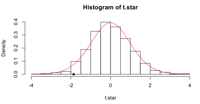 We can get some quantiles.
> quantile(t.star, c(.025,.05,.5,.950,.975))
       2.5%          5%         50%         95%       97.5%
-1.92422717 -1.65896181 -0.07050922  1.62722956  2.09215955
The simulation p-value is obtained as previously.
> mean(t.star <= -1.8608)         # one-tailed
[1] 0.031
> mean(abs(t.star) >= 1.8608)     # two-tailed
[1] 0.065
Our reference two-tailed p-value from the "actual" t-test is 0.079.
Automating It With boot()
Let's bootstrap the actual t-test. (Btw, you can bet I'm typing this into
a script window!)
> boot.tee = function(data, i) {
+    d = data[i,]
+    c(t.test(d$extra[1:10], d$extra[11:20], var.eq=T)$statistic,
+      t.test(d$extra[1:10], d$extra[11:20], var.eq=T)$p.value)
+ }
> boot.out = boot(data=sleep, statistic=boot.tee, R=1000)
Here's the explanation. First, I defined a function called boot.tee, which is
a function of the data and i. Our boot.tee function will find out what
the "data" are when we tell that to boot(). I
handed each permuted value of the
data to a variable called d. (I don't know if this is standard, but it's a
trick I learned in Zieffler, et al, and I thought it was very clever.)
Then I created a vector
containing two output values: the t-value from the t-test, and p-value from
that test. Notice when I did that, I did not use a formula interface, DV~IV.
I would do that if I was starting with the assumption that the alternative
hypothesis is true, as that would cause group 1 values to be bootstrapped
from group 1, and group 2 values to be bootstrapped from group 2 of the
original data. In other words, when the data frame is permuted, all columns of
it are permuted, so scores (extra) remain paired with the group from whence
they came in any given row of the permuted data. Instead, I was starting with
the assumption that the null
hypothesis is true. I let boot permute the data frame into a random order,
jumbling up the rows in the process,
and then I tested the first ten scores against the last ten.
If I want to check to see if this function is working properly, I can run
it on the original data frame and see if it gives me the right answers.
> boot.tee(sleep)
          t
-1.86081347  0.07918671
Then I ran the boot() function (and immediately got an error because it's
a new day, and I forgot to load the "boot" library). Let's see what we got.
> boot.out

ORDINARY NONPARAMETRIC BOOTSTRAP

Call:
boot(data = sleep, statistic = boot.tee, R = 1000)

Bootstrap Statistics :
       original    bias    std. error
t1* -1.86081347 1.8628096   1.0646010
t2*  0.07918671 0.4121642   0.2867875
I get output for both items I calculated as part of the statistic. First, t1*
is the t-value, and second, t2* is the p-value. The first thing I'm told is
what the values are when the function is run on the original data ("original").
Then I'm told how far off the bootstrapped values are from that ("bias"), on
the average. Finally, I'm given the standard deviation of the 1000 bootstrapped
value ("std. error").
> summary(boot.out$t)                  # boot.out$t is a matrix in this case
       V1                  V2
 Min.   :-4.029412   Min.   :0.0007866
 1st Qu.:-0.685015   1st Qu.:0.2468949
 Median :-0.011462   Median :0.4913727
 Mean   : 0.001996   Mean   :0.4913510
 3rd Qu.: 0.722583   3rd Qu.:0.7358411
 Max.   : 3.242622   Max.   :1.0000000
The actual bootstrapped values are inside boot.out in a variable called t, so
I asked for a summary of that. V1 is the first thing I calculated (t-value),
and V2 is the second thing I calculated (p-value). Notice that the means in both
cases are equal to original + bias from the first output. For finer grained info,
we'll run quantile(), and we MUST remember to ask
for a specific column of the t matrix. Otherwise, we'll be getting quantiles
from the t-values and p-values all mixed together. Not useful!
> quantile(boot.out$t[,1], c(.025,.05,.5,.95,.975))
       2.5%          5%         50%         95%       97.5%
-2.02421421 -1.75560123 -0.01146238  1.77771580  2.10951478
The result is very similar to what we got in t.star, but not exactly the same
because this was a new set of permutations of the data. The p-values also
differ a bit.
> mean(boot.out$t[,1] < -1.8608)       # one-tailed
[1] 0.038
> mean(abs(boot.out$t[,1]) >= 1.8608)  # two-tailed
[1] 0.081
Note: There is a function in
the "boot" library called boot.ci(), but the
output doesn't agree with above, and I'm not sure why. As usual, the help
page wasn't much help. The explanation is NOT that the output object is a
matrix, because it doesn't work (for me) if only one stat is calculated. So
I don't use this function!
Here is an example of how to use it from stackoverflow.com.
> x <- rnorm(100, 1, .5)
> b <- boot(x, function(u,i) mean(u[i]), R = 999)
> boot.ci(b, type = c("norm", "basic", "perc"))
BOOTSTRAP CONFIDENCE INTERVAL CALCULATIONS
Based on 999 bootstrap replicates

CALL :
boot.ci(boot.out = b, type = c("norm", "basic", "perc"))

Intervals :
Level      Normal              Basic              Percentile
95%   ( 0.962,  1.206 )   ( 0.961,  1.205 )   ( 0.963,  1.206 )
Calculations and Intervals on Original Scale

> quantile(b$t,c(.025,.975))           # for comparison
     2.5%     97.5%
0.9632601 1.2059236
Seems to work here. Didn't work above. Good luck!
Note: When a test statistic such as a Student's t is bootstrapped,
Zieffler, Harring, and Long (2011, see refs) call
this bootstrapping using a pivot statistic (p. 163). They imply that it's a
bit safer than the parametric bootstrap, which is outlined below, because
fewer population parameters must be "known."
Bootstrapping The Difference in Means
Assuming the Null Hypothesis is True
First, we'll combine all the DV values into one "population" and pull
both bootstrap samples from that. Our obtained value for the difference in
means is 1.58, for reference.
> mean.diff = function(data, i) {
+    d = data[i,]
+    mean(d$extra[11:20]) - mean(d$extra[1:10])
+ }

> mean.diff(sleep)      # test function on original data
[1] 1.58

> boot.out = boot(data=sleep, statistic=mean.diff, R=1000)

> quantile(boot.out$t, c(.025,.05,.5,.95,.975))
    2.5%       5%      50%      95%    97.5%
-1.72025 -1.44050 -0.04000  1.44050  1.67025

> mean(boot.out$t >= 1.58)        # one-tailed p-value
[1] 0.035
> mean(abs(boot.out$t) >= 1.58)   # two-tailed p-value
[1] 0.068
The bootstrapped 95% CI on the mean difference values consistent with the null
is -1.72 to 1.67. This interval includes the reference value.
In this case, we handed our function the data (to be specified in boot) and
an indexing variable i, we passed off the current (ith) bootstrap of the
data to d. The data is to be a data frame, so two indices are needed on data[i,].
The first index, i, contains a bootstrapped sample of the rows 1:20. The second
is blank, which means all columns. Since the rows of the data have now been
randomly permuted, or actually randomly bootstrap sampled, any arbitrary 10
values can be used to calculate the first mean, and the other 10 values the
second mean. The easiest way is 11:20 for the first mean and 1:10 for the
second mean, or vice versa. (Note: This method is illustrated by Zieffler
et al, p. 160.)
The same procedure without boot() would look
like this.
> data = sleep
> R = 1000
> results = numeric(R)
> for (i in 1:R) {
+    indices = sample(1:20, size=20, replace=T)
+    d = data[indices,]
+    results[i] = mean(d$extra[11:20]) - mean(d$extra[1:10])
+ }
> quantile(results, c(.025,.05,.5,.95,.975))
    2.5%       5%      50%      95%    97.5%
-1.66000 -1.40150 -0.00500  1.41050  1.70025
> mean(abs(results) >= 1.58)
[1] 0.067
Not Assuming the Null Hypothesis is True
This time we will take bootstrap samples from the individual groups. For
reference, the obtained mean difference is 1.58, and the parametric 95%
confidence interval is -0.20 to +3.36.
> mean.diff = function(data, i) {
+    d = data[i,]
+    mean(d$extra[d$group==2]) - mean(d$extra[d$group==1])
+ }

> mean.diff(sleep)      # test function on original data
[1] 1.58

> boot.out = boot(data=sleep, statistic=mean.diff, R=1000, strata=sleep$group)

> quantile(boot.out$t, c(.025,.05,.5,.95,.975))
    2.5%       5%      50%      95%    97.5%
-0.03000  0.23950  1.61000  2.87000  3.09075

> mean(boot.out$t <= 0)      # one-tailed p-value
[1] 0.028
The bootstrapped 95% CI on the mean difference is -0.03 to 3.09, a little
narrower than the parametric value. I've run this many times, and the lower
bound of the CI jumps back and forth across 0. Even at R=10000, the lower
bound can't quite decide which side of 0 it wants to be on. So this is a
close one.
When the order of rows in the data frame is permuted (bootstrapped), the
group information remains with the data values. So this time the mean.diff
function calculates the difference between a mean of values that came from
group 2 and a mean of values that came from group 1. The strata= option is
not actually necessary to make the procedure run and give an answer, but it
seems to make a slight difference in the width of the CI, so I'm not
sure how it's used, but it should be included to tell the procedure that the
two groups are being sampled separately. (Note: This method is illustrated by
Zieffler et al, p. 190.)
The same procedure without boot() would look
like this.
> data = sleep
> R = 1000
> results = numeric(R)
> for (i in 1:R) {
+    indices = sample(1:20, size=20, replace=T)
+    d = data[indices,]
+    results[i] = mean(d$extra[d$group==2]) - mean(d$extra[d$group==1])
+ }
> quantile(results, c(.025,.05,.5,.95,.975))
     2.5%        5%       50%       95%     97.5%
0.0248750 0.1899048 1.5415862 2.9043119 3.1559799
> mean(results <= 0)
[1] 0.024
Important note: How do you get a poor result from a bootstrap? Use small
samples. While I've used a small sample case above to illustrate the methods,
you should probably be wary of using bootstrap in such cases.
Permutation and Randomization Tests: The Jackknife
I will use the sleep data to illustrate our
next topic as well, which is permutation tests.
The logic behind a permutation test is straightforward. It says, "Okay, these
are the twenty (in this example) scores we got, and the way they are divided up
between the two groups is one possible permutation of them. There are, in
fact...
> choose(20,10)
[1] 184756
...possible permutations (technically combinations--but same idea) of these
data into two groups of ten, and each is equally likely to occur if we were to
pick one at random out of a hat. Most of these permutations would give no or
little difference between the group means, but a few of them would give large
differences. How extreme is the obtained case?" In other words, the logic of
the permutation test is quite similar to the logic of the t-test. If the
obtained case is in the most extreme 5% of possible results, then we reject the
null hypothesis of no difference between the means (assuming we were looking at
differences between means). The advantage of the permutation test is, it does
not make any assumption about normality, and in fact, doesn't make any
assumption at all about parent distributions. Furthermore, a permutation test
is generally more powerful than a "traditional" nonparametric test.
The disadvantage of a permutation test is the number of permutations that
must be generated. Even small samples, as we have here, will choke a typical
desktop computer with repetitive calculations. Therefore, instead of generating
all possible permutations, we generate only a random sample of them. This
procedure is often called a "randomization test" instead of a permutation test.
Let's see the elephant, and then I'll explain.
> ### Begin by cleaning up your workspace, if you haven't already.
> R = 1000
> scores = sleep$extra
> t.star = numeric(R)
> for (i in 1:R) {
+    index = sample(1:20, size=10, replace=F)
+    group1 = scores[index]
+    group2 = scores[-index]
+    t.star[i] = t.test(group1, group2, var.eq=T)$statistic
+ }
First, we set the number of
sims (replications, resamplings) to 1000. Then we made a copy of the data, which
was really unnecessary. Then we established a storage vector for the results of
the sims. Then we began looping. Inside the loop, we took a random sample of the
vector 1 to 20, without replacement, and stored that in an object called
"index". These index values were then used to extract the first resampled group
of scores. The second group of scores was extracted using a trick, which in
words goes, "for group two take all the scores that are not indexed by the
values in index." In other words, put the remaining scores in group two. Then we
did the t-test and stored the test statistic (t-value). It now remains to
compare those simulated t-values to the one we obtained above when we did the
actual t-test.
> mean(abs(t.star) >= 1.8608)          # two-tailed test
[1] 0.072
The resampling scheme tells us that a little more than 7% of the sims gave us a
result as extreme or more extreme than the obtained case. This is the p-value
resulting from the randomization test. We can see that it is pretty close to the
p-value obtained in the actual t-test above (.0794). The difference may be
nothing more than random noise. (Note: Once again, your result will be
different due to the randomization done by sample().)
The bootstrap method simulates random sampling from a population. The
randomization method, sometimes called jackknife resampling, simulates random
assignment to groups. It's usually considered the preferred method if your
subjects are volunteers or you snatched them out of the hallway during
change of classes.
Another Way
There are as many ways to do randomization tests as there are statistics
you can think up to assess the difference between the groups. Here is another
way. Notice in this case I've use a different, but equally effective, method
of resampling as well. I merely rearrange (permute) the scores and use the
original grouping variable to index them.
> R = 1000
> scores = sleep$extra
> groups = sleep$group
> mean.diff = numeric(1000)
> for (i in 1:R) {
+    perm.scores = sample(scores, size=20)
+    mean.diff[i] = diff(tapply(perm.scores, groups, mean))
+ }
> tapply(scores, groups, mean)
   1    2
0.75 2.33
> 2.33 - .75            # the obtained difference
[1] 1.58
> mean(abs(mean.diff) >= 1.58)
[1] 0.086
The result is similar. We'd get a narrower range of results if the
samples were larger.
Paired Scores
"Hey! These are paired scores. Deal with that!" First, let's get some
reference info from the standard t-test for paired scores.
> t.test(extra ~ group, data=sleep, paired=T)

	Paired t-test

data:  extra by group
t = -4.0621, df = 9, p-value = 0.002833
alternative hypothesis: true difference in means is not equal to 0
95 percent confidence interval:
 -2.4598858 -0.7001142
sample estimates:
mean of the differences
                  -1.58
The logic behind randomization in this case is that it is a matter of chance
which of the paired scores occurred in the control group and which occurred in
the treatment group. In other words, when we look at the sign on the difference
scores, it's a coin flip as to whether than sign will be positive or negative.
The difference scores are...
> diffs = sleep$extra[1:10] - sleep$extra[11:20]
> diffs
 [1] -1.2 -2.4 -1.3 -1.3  0.0 -1.0 -1.8 -0.8 -4.6 -1.4
...and a lot of them are negative, but the null hypothesis says that's just
dumb luck. Given that those are the difference scores, it's a matter of pure
chance what sign they have. And there is the randomization we need to justify
a randomization test.
> R = 1000                                       # we'll do 1000 sims
> absdiffs = abs(diffs)                          # strip the signs
> results = numeric(R)                           # create a storage vector
> for (i in 1:R) {                               # begin looping
+    sign = sample(c(1,-1), 10, replace=T)       # get 10 random signs
+    results[i] = mean(absdiffs * sign)          # get mean of diffs with new signs
+ }
> quantile(results, c(.025,.975))                # 95% of them fall in what interval?
 2.5% 97.5%
-1.16  1.14
> mean(abs(results) >= 1.58)                     # two-tailed p-value
[1] 0.006
The result is not too different from what the t-test revealed. You can
completely clear your workspace now. We are done with "sleep".
About Those p-Values
Some sources propose that the p-values derived as above are ever so slightly
too small and that a correction should be applied that can be calculated like
this.
p.corrected = (pR + 1) / (R + 1)
Where p is the probability as calculated above and R is the number of
replications. With R = 1000, the largest correction this will ever result in
is less than .001, which is undoubtedly well within the boundaries of
uncertainty on the p-value anyway. To apply a correction to the third or
fourth decimal place of a value that's probably not entirely accurate in the
second decimal place strikes me as being a little fussy. But there you have it.
Use it as you see fit. With a smaller number of reps, it could be important.
Note on terminology: As we are taking a random sample of possible
permutations of the data in the jackknife, jackknife resampling can reasonably
be referred to as Monto Carlo resampling, and often is.
Bootstrapped Confidence Intervals
Bootstrap resampling is useful for estimating confidence intervals from
samples when the sample is from an unknown (and clearly nonnormal) distribution.
The data set "crabs" in the MASS package supplies an example. We will look at
the carapace length of blue crabs.
> data(crabs, package="MASS")
> cara = crabs$CL[crabs$sp=="B"]
> summary(cara)
   Min. 1st Qu.  Median    Mean 3rd Qu.    Max.
  14.70   24.85   30.10   30.06   34.60   47.10
> length(cara)
[1] 100
> qqnorm(cara)                         # not shown
Hmmmm, that looks reasonably normal to me, but who can say for sure? So to get
a 95% CI for the mean, we will use a bootstrap scheme rather than methods based
on a normal distribution. But just for reference purposes, the normal
distribution method would give the following result.
> t.test(cara)$conf.int
[1] 28.68835 31.42765
attr(,"conf.level")
[1] 0.95
The procedure is to take a large number of bootstrap samples and
to examine the desired statistic.
> R = 1000
> boot.means = numeric(R)
> for (i in 1:R) {
+    boot.sample = sample(cara, 100, replace=T)
+    boot.means[i] = mean(boot.sample)
+ }
> quantile(boot.means, c(.025,.975))
    2.5%    97.5%
28.71027 31.37937
The bootstrapped CI is reasonably close to the one obtained by traditional
methods, so the normal approximation seems to be reasonable for these data.
Extension to more complex problems is straightforward.
Doing It With boot()
I have to admit that using boot() may be just
a smidge easier in this case.
> boot.means = function(cara, i) {mean(cara[i])}
> boot.out = boot(data=cara, statistic=boot.means, R=1000)
> quantile(boot.out$t, c(.025,.975))
    2.5%    97.5%
28.75858 31.39305
But certainly no less cryptic! It may also be useful just too look at the
output of boot() directly.
> boot.out

ORDINARY NONPARAMETRIC BOOTSTRAP

Call:
boot(data = cara, statistic = boot.means, R = 1000)

Bootstrap Statistics :
    original   bias    std. error
t1*   30.058 0.015603   0.6902185
The value "original" is the mean of the original data
vector "cara". The value "bias" gives the difference between "original" and the
mean of the bootstrapped values for this statistic. Clearly, "bias" ought to be
close to zero. The value "std. error" is the standard deviation of the
bootstrapped means.
Bootstrapping is more usefully applied to statistics like the median, for
which there is no formula for CIs when the distribution is not normal.
> boot.medians = function(cara, i) {median(cara[i])}
> boot.out = boot(data=cara, statistic=boot.medians, R=1000)
> quantile(boot.out$t, c(.025,.975))
 2.5% 97.5%
27.85 32.40
> boot.out

ORDINARY NONPARAMETRIC BOOTSTRAP

Call:
boot(data = cara, statistic = boot.medians, R = 1000)

Bootstrap Statistics :
    original  bias    std. error
t1*     30.1 0.08145    1.461501
Clean up your workspace. It's a mess!
The Parametric Bootstrap
So far, and in future sections as well, what we've been doing is called the
nonparametric bootstrap, because no assumptions are being made about population
parameters. We will use some data from the MASS package to illustrate an
alternative method called the parametric bootstrap.
> data(birthwt, package="MASS")
> head(birthwt)
   low age lwt race smoke ptl ht ui ftv  bwt
85   0  19 182    2     0   0  0  1   0 2523
86   0  33 155    3     0   0  0  0   3 2551
87   0  20 105    1     1   0  0  0   1 2557
88   0  21 108    1     1   0  0  1   2 2594
89   0  18 107    1     1   0  0  1   0 2600
91   0  21 124    3     0   0  0  0   0 2622

> bw = birthwt[,c("smoke","bwt")]      # we need only these two columns
> bw$smoke = factor(bw$smoke, labels=c("no","yes"))
> summary(bw)
 smoke          bwt
 no :115   Min.   : 709
 yes: 74   1st Qu.:2414
           Median :2977
           Mean   :2945
           3rd Qu.:3487
           Max.   :4990
>rm(birthwt)
The data show birthweights (bwt) in grams of babies born to mothers who
smoked and mothers who did not smoke. The obvious point of interest is,
what's the difference, if any, in the mean birthweights for the two groups?
Let's look at the data.
> with(bw, tapply(bwt, smoke, mean))
      no      yes
3055.696 2771.919
> with(bw, tapply(bwt, smoke, var))
      no      yes
566492.0 435118.2
> plot(density(bw$bwt[bw$smoke=="yes"]))              # not shown
> lines(density(bw$bwt[bw$smoke=="no"]),col="red")
The means are different by a bit more than 280 grams. The variances are also
different, but not too much. The last two lines of code plot overlapping
kernel density
estimates of the distributions, which show that both of them are mound shaped
and not too terribly different from normal. Thus, we will assume that both
groups were sampled from the same normal distribution that has parameters
equal to the sample mean and variance. (We are assuming the null hypothesis
is true, and that our "bwt" variable is sampled from a single normal
distribution.)
The first step is to create a DV that consists of standardized values as if
they were drawn from a single population with a mean of 0 and a standard
deviation of 1. This can be done with the scale()
function.
> bw$z.bwt = scale(bw$bwt)
Now we'll investigate the difference between the two groups on this variable.
> with(bw, tapply(z.bwt, smoke, mean))
        no        yes
 0.1523672 -0.2367869
> with(bw, diff(tapply(z.bwt, smoke, mean)))
       yes
-0.3891541
The difference is almost four tenths of a standard deviation. The syntax for
the parametric bootstrap is:
boot(data, statistic, R, sim="parametric", ran.gen)
The last two options are new. One of them obviously tells R that we want a
parametric bootstrap. The other one is another function that we have to write
to generate Monte Carlo samples from the standard normal distribution
(assuming it is the normal distribution that we have decided fits our data).
bwt.gen = function(data, mle) {
   rnorm(n=length(data))
}
I have no idea why the mle is necessary, but it is. As usual, we also need the
function that calculates our test statistic.
mean.diff = function(data, i) {
   mean(data[1:115]) - mean(data[116:189])
}
Since we've generated a random vector of standard scores in bwt.gen, I just
took the difference in means between the first 115 of them (representing
nonsmokers) and the last 74 of them (representing smokers). Once those
functions are executed and in the workspace, we can run boot().
> boot.out = boot(data=bw$z.bwt, statistic=mean.diff, R=1000, sim="parametric", ran.gen=bwt.gen)
The results are in the usual place.
> boot.out

PARAMETRIC BOOTSTRAP

Call:
boot(data = bw$z.bwt, statistic = mean.diff, R = 1000, sim = "parametric",
    ran.gen = bwt.gen)

Bootstrap Statistics :
     original    bias    std. error
t1* 0.9683415 -0.965374   0.1527679

> summary(boot.out$t)
       V1
 Min.   :-0.553122
 1st Qu.:-0.099277
 Median : 0.006685
 Mean   : 0.002968
 3rd Qu.: 0.104059
 Max.   : 0.504965

> quantile(boot.out$t, c(.025,.975))   # does not contain 0.3891541, so yay!
      2.5%      97.5%
-0.3040931  0.3042744

> mean(abs(boot.out$t) >= 0.3891541)   # two-tailed p-value
[1] 0.011
For the record, the parametric p-value from the t-test is .0087.
It seems to me that "parametric bootstrap" is just a new name for
Monte Carlo simulation. How are they different?
Bootstrapping a Regression Analysis
First, thanks to John Fox for a very clear example of how to use boot() here, which I found in a document posted
here. Here is where the boot()
function is going to shine, I have to admit. We will look at a problem that we
also examine in the Multiple Regression tutorial,
in which we attempt to predict life expectancy by U.S. state using various
predictors (1977 data).
> states = state.x77
> states = as.data.frame(states)                           # must be a data frame
> colnames(states)[c(4,6)] = c("Life.Exp","HS.Grad")       # fix some variable names
> lm(Life.Exp ~ Murder + HS.Grad + Frost, data=states)     # for reference

Call:
lm(formula = Life.Exp ~ Murder + HS.Grad + Frost, data = states)

Coefficients:
(Intercept)       Murder      HS.Grad        Frost
  71.036379    -0.283065     0.049949    -0.006912
First, we define a function to get the statistic(s) we want, which are the
regression coefficients.
> boot.states = function(states, i) {
+    mod = lm(Life.Exp ~ Murder + HS.Grad + Frost, data=states[i,])
+    coefficients(mod)
+ }
Once again, the data are not just "states" but states[i,] from the ith
iteration of the bootstrap. Now it remains to run
boot() and examine the output.
> boot.out = boot(data=states, statistic=boot.states, R=1000)
> boot.out

ORDINARY NONPARAMETRIC BOOTSTRAP

Call:
boot(data = states, statistic = boot.states, R = 1000)

Bootstrap Statistics :
        original        bias    std. error
t1* 71.036378813 -0.1117470290 1.111679000       # intercept
t2* -0.283065168  0.0050440366 0.040044342       # Murder slope
t3*  0.049948704  0.0009847503 0.017462937       # HS.Grad slope
t4* -0.006911735  0.0002284539 0.003021178       # Frost slope

> summary(boot.out$t)
       V1              V2                V3                 V4
 Min.   :66.42   Min.   :-0.3927   Min.   :0.002082   Min.   :-0.016386
 1st Qu.:70.29   1st Qu.:-0.3056   1st Qu.:0.039119   1st Qu.:-0.008695
 Median :71.03   Median :-0.2824   Median :0.050579   Median :-0.006672
 Mean   :70.92   Mean   :-0.2780   Mean   :0.050933   Mean   :-0.006683
 3rd Qu.:71.69   3rd Qu.:-0.2548   3rd Qu.:0.061776   3rd Qu.:-0.004735
 Max.   :73.49   Max.   :-0.1007   Max.   :0.122853   Max.   : 0.003244

> quantile(boot.out$t[,2], c(.025,.975))         # 95% CI for Murder slope
      2.5%      97.5%
-0.3452561 -0.1883249
> quantile(boot.out$t[,3], c(.025,.975))         # compare this to boot.ci() answer below
      2.5%      97.5%
0.01702089 0.08657885

> confint(lm(Life.Exp ~ Murder + HS.Grad + Frost, data=states))      # parametric CIs for comparison
                  2.5 %       97.5 %
(Intercept) 69.05717472 73.015582905
Murder      -0.35700149 -0.209128849
HS.Grad      0.01935043  0.080546980
Frost       -0.01183825 -0.001985219

> boot.ci(boot.out, type="perc", index=3)        # still doesn't give quite the right answer
BOOTSTRAP CONFIDENCE INTERVAL CALCULATIONS
Based on 1000 bootstrap replicates

CALL :
boot.ci(boot.out = boot.out, type = "perc", index = 3)

Intervals :
Level     Percentile
95%   ( 0.0169,  0.0867 )
Calculations and Intervals on Original Scale
Now, clean up your workspace in preparation for the next and final section,
but KEEP the states data frame. We're going to use it again.
Resampling a Oneway ANOVA
We will begin by adding a factor, census region, to the "states" data frame,
which hopefully you still have left over from the last section. We're going to
change the value labels on the fly because, once again, spaces in the variable
names! Whose idea was that? (Note: state.region is a built-in data object.)
> states$Region = factor(state.region, labels=c("Northeast","South","Midwest","West"))
> summary(states)
   Population        Income       Illiteracy       Life.Exp         Murder
 Min.   :  365   Min.   :3098   Min.   :0.500   Min.   :67.96   Min.   : 1.400
 1st Qu.: 1080   1st Qu.:3993   1st Qu.:0.625   1st Qu.:70.12   1st Qu.: 4.350
 Median : 2838   Median :4519   Median :0.950   Median :70.67   Median : 6.850
 Mean   : 4246   Mean   :4436   Mean   :1.170   Mean   :70.88   Mean   : 7.378
 3rd Qu.: 4968   3rd Qu.:4814   3rd Qu.:1.575   3rd Qu.:71.89   3rd Qu.:10.675
 Max.   :21198   Max.   :6315   Max.   :2.800   Max.   :73.60   Max.   :15.100
    HS.Grad          Frost             Area              Region
 Min.   :37.80   Min.   :  0.00   Min.   :  1049   Northeast: 9
 1st Qu.:48.05   1st Qu.: 66.25   1st Qu.: 36985   South    :16
 Median :53.25   Median :114.50   Median : 54277   Midwest  :12
 Mean   :53.11   Mean   :104.46   Mean   : 70736   West     :13
 3rd Qu.:59.15   3rd Qu.:139.75   3rd Qu.: 81162
 Max.   :67.30   Max.   :188.00   Max.   :566432

> boxplot(Income ~ Region,states)                # not shown
> with(states, tapply(Income, Region, mean))
Northeast     South   Midwest      West
 4570.222  4011.938  4611.083  4702.615
> with(states, tapply(Income, Region, sd))
Northeast     South   Midwest      West
 559.0771  605.4505  283.0825  663.9004
The relationship we are interested in is Income by Region (in case you didn't
guess). It looks like we have some pretty substantial differences here,
particularly between the South and the other regions. It also looks like we
have heterogeneous variances.
Monte Carlo Simulation
Let's use a Monte Carlo simulation to get an F.star distribution assuming the
null hypothesis is correct, and the four regions are actually samples from one
and the same population, and assuming normality and homogeneity as well.
> data.star = states$Income
> mean.star = mean(data.star)
> sd.star = 555.0118              # the pooled standard deviation obtained from aov()
> IV.star = factor(rep(c("NE","S","MW","W"), times=c(9,16,12,13)))
> R = 1000
> F.star = numeric(R)
> for (i in 1:R) {
+    DV.star = c(rnorm(9, mean=mean.star, sd=sd.star),
+                rnorm(16, mean=mean.star, sd=sd.star),
+                rnorm(12, mean=mean.star, sd=sd.star),
+                rnorm(13, mean=mean.star, sd=sd.star))    # a little silly, but...
+    F.star[i] = oneway.test(DV.star ~ IV.star, var.eq=T)$statistic
+ }
We should now have our simulated F-distribution (F.star) for df=3,46. I'll plot
it and then draw the theoretical F(3,46)-distribution over top of it.
> hist(F.star, breaks=30, prob=T, xlim=c(0,7), ylim=c(0,.8))
> points(x<-seq(0,7,.1), y=df(x,3,46), type="b", cex=.6, col="red")
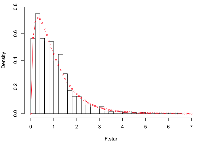 They are very similar, which is not surprising given the way F.star was
created. For reference:
They are very similar, which is not surprising given the way F.star was
created. For reference:
> oneway.test(Income~Region, data=states, var.eq=T)

	One-way analysis of means

data:  Income and Region
F = 4.687, num df = 3, denom df = 46, p-value = 0.006136

> mean(F.star >= 4.687)                # p-value
[1] 0.006
That's as close as we could come given 1000 sims. Let's do it again assuming
equal means but not assuming equal variances. For reference:
> oneway.test(Income ~ Region, data=states)

	One-way analysis of means (not assuming equal variances)

data:  Income and Region
F = 4.2638, num df = 3.000, denom df = 22.377, p-value = 0.01596

> R = 1000
> F.star = numeric(R)
> for (i in 1:R) {
+    DV.star = c(rnorm(9, mean=mean.star, sd=559.08),
+                rnorm(16, mean=mean.star, sd=605.45),
+                rnorm(12, mean=mean.star, sd=283.08),
+                rnorm(13, mean=mean.star, sd=663.90))
+    F.star[i] = oneway.test(DV.star ~ IV.star, var.eq=T)$statistic
+ }

> hist(F.star, breaks=30, prob=T, xlim=c(0,8), ylim=c(0,1))
> points(x<-seq(0,7,.1), y=df(x,3,46), type="b", cex=.6, col="red")
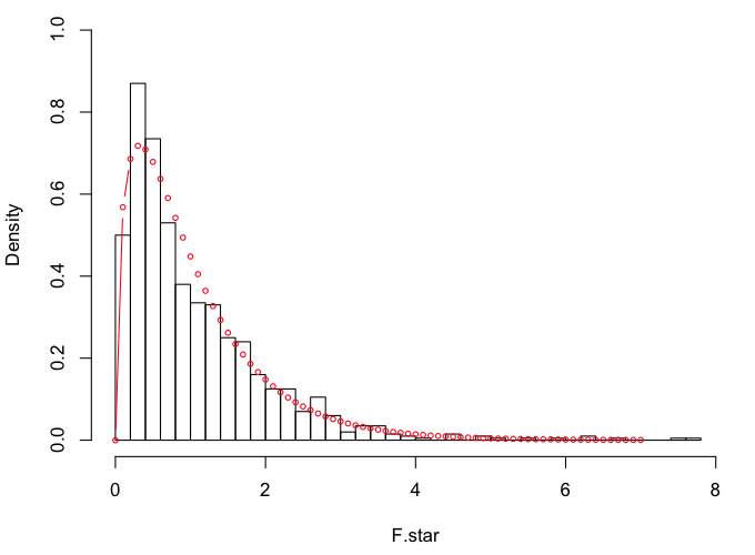 Looks like we might be a little heavier in the tails this time.
> qf(.95, 3, 46)
[1] 2.806845
> quantile(F.star, .95)                # okay, maybe not
    95%
2.78404

> mean(F.star >= 4.2638)               # p-value
[1] 0.013
Randomization Test
One key assumption of the randomization test, not previously mentioned, is
exchangeability. Basically, this means that a subject who ended up in one group
could just have easily have ended up in some other group. The only way to
guarantee exchangeability is to do random assignment to groups. Thus, the
randomization test is often reserved for true, randomized experiments. With
intact groups, it's hard to say that a Missourian could just have easily been
a Californian, or that California could just as easily have ended up in the
Midwest. (They do have some rather "interesting" earthquakes out there. Just
saying, speaking as a person who used to live there!) Nevertheless, just to
illustrate the method, we're going to assume exchangeability.
> income = states$Income          # just making the data a little more accessible
> region = states$Region
> R = 1000                        # 1000 reps (good thing we're not doing pushups!)
> results = numeric(R)            # a place to store the results
> for (i in 1:R) {
+    permuted.income = sample(income, size=50, replace=F)
+    results[i] = oneway.test(permuted.income ~ region)$statistic
+ }
> mean(results >= 4.2638)         # F = 4.2638 is the result from the real data
[1] 0.022
Assuming the null hypothesis is true, and permuting (resampling without
replacement) the income values 1000 times, we find the probability of getting a
result greater than or equal to the observed one is 0.022. The test was done
without assuming homogeneity of variance.
Let's Try boot()ing It
Zieffler et al suggest that a good statistic to bootstrap for an ANOVA is
the effect size, eta-squared. Others have suggested the treatment sum of squares,
the treatment mean square, and the variance of the treatment means. As these are
all functions of F and the degrees of freedom, it seems to me that they should
give the same result as bootstrapping F (degrees of freedom being constants for
any given problem). Let's find out.
> aov(income ~ region)
Call:
   aov(formula = income ~ region)

Terms:
                  region Residuals
Sum of Squares   4331342  14169750
Deg. of Freedom        3        46

Residual standard error: 555.0118
Estimated effects may be unbalanced
> 4331342/3
[1] 1443781
> var(tapply(income, region, mean))
[1] 97939.1
First we get some reference values. SST = 4331342. MST = 1443781. VarT =
97939.1. I'm going to store these, because I don't want to have to remember
them.
> SST = 4331342
> MST = 1443781
> VarT = 97939.1
> Eta2 = 4331342 / (4331342 + 14169750)     # eta-sq = 0.2341128
> Fobs = (4331342/3) / (14169750/46)        # assuming homogeneity, F = 4.687021
I'm having second thoughts about the variance of the treatment means, given
that this is an unbalanced design. I think it would work if the design were
balanced. Now we have to write a function, to be used by the bootstrap, that
calculates all these things. To make life easier, I'm going to get rid of the
original data frame, make a new one from just the variables we're using, and
then erase those from the workspace.
> rm(states)
> states = data.frame(income, region)
> rm(income, region)
Okay, here we go!
> SS = function(x)  sum(x^2) - sum(x)^2/length(x)     # a function for sum of squares
> boot.states = function(data,i) {
+    d = data[i,]
+    aov.out = aov(d$income ~ states$region)
+    SST.star = SS(d$income) - SS(aov.out$residuals)
+    MST.star = SST.star / 3
+    VarT.star = var(tapply(d$income, states$region, mean))
+    Eta2.star = SST.star / SS(d$income)
+    F.star = MST.star / (SS(aov.out$residuals)/46)
+    c(SST.star, MST.star, VarT.star, Eta2.star, F.star)
+ }
> boot.states(states)             # looks like our function passes the test
[1] 4.331342e+06 1.443781e+06 9.793910e+04 2.341127e-01 4.687020e+00
> bout = boot(data=states, statistic=boot.states, R=1000)
> summary(bout$t)
       V1                V2                V3               V4                  V5
 Min.   :   4453   Min.   :   1484   Min.   :  3649   Min.   :0.0002858   Min.   :0.004383
 1st Qu.: 460119   1st Qu.: 153373   1st Qu.: 75190   1st Qu.:0.0260488   1st Qu.:0.410097
 Median : 881114   Median : 293705   Median :112246   Median :0.0495693   Median :0.799704
 Mean   :1145724   Mean   : 381908   Mean   :120906   Mean   :0.0632042   Mean   :1.088080
 3rd Qu.:1533472   3rd Qu.: 511157   3rd Qu.:156216   3rd Qu.:0.0879430   3rd Qu.:1.478482
 Max.   :9006160   Max.   :3002053   Max.   :390738   Max.   :0.3856425   Max.   :9.624990
Alright! Drove myself a little crazy with that one for awhile! Until I discovered
that the proper ANOVA was not aov.out = aov(d$income ~ d$region). That would be
assuming the null hypothesis is false. We are assuming the null hypothesis is
true, so we have to do the ANOVA against the original (unbootstrapped)
arrangement of region. Same thing for the variances of the treatment means (of
course). Zieffler also calculated eta-squared from the original
SS Total rather than the bootstrapped one, as I have above. I'm not sure what
the justification is for that. Now for the moment of truth.
> mean(bout$t[,1] >= SST)
[1] 0.019
> mean(bout$t[,2] >= MST)
[1] 0.019
> mean(bout$t[,3] >= VarT)
[1] 0.031
> mean(bout$t[,4] >= Eta2)
[1] 0.009
> mean(bout$t[,5] >= Fobs)
[1] 0.009
Here's what we've learned. Bootstrapping SST and MST give the same result.
That's not surprising since one is a linear transform of the other. The
variance of the group means would also give the same result if the design
were balanced, because it is MST/n per group in those cases. In the many runs
of this I did, the bootstrap of the treatment variances consistently resulted
in the highest p-value, in this unbalanced case. The unbalanced
design has, appropriately, cost us a little power. Bootstrapping
eta-squared gives the same result as SST and MST if the original SS
Total is used to calculate it (as per Zieffler et al). If not, it gives the same
result as bootstrapping
the F statistic (as here and as expected, as it is a linear transform of F).
Bootstrapping the F statistic consistently gives a
slightly smaller p-value than bootstrapping SST and MST (and Eta2 if the original
SS Total is used to calculate it).
revised 2016 March 6; updated March 8
| Table of Contents
| Function Reference
| Function Finder
| R Project |
|