
| Table of Contents
| Function Reference
| Function Finder
| R Project |
HIERARCHICAL REGRESSION
Preliminaries
I am not well read on the topic of hierarchical regression, so for details,
especially on theory, you'd be well advised to consult another source. I've
found a textbook by Keith (2006) to be very helpful. It is well written and
gets to the point without getting bogged down in a lot of mathematical finery.
What theory I do present here is adapted from that source. I'm also going to
borrow a data set from him. Kieth, by the way, refers to hierarchical
regression as sequential regression. Other resources I found helpful were
Petrocelli (2003), who discussed common problems with and misuses of
hierarchical regression, and Lewis (2007), who compared hierarchical with
stepwise regression.
I felt it necessary to create this tutorial to support another
on Unbalanced Factorial Designs. As we'll find
out, Type I sums of squares, the R default in ANOVA, does something similar
to hierarchical regression, but not quite exactly. There is a difference in
the error terms that are used, which I'll discuss below.
- Lewis, M. (2007). Stepwise versus hierarchical regression: Pros and cons.
Paper presented at the annual meeting of the Southwest Educational Research
Association, February 7, 2007, San Antonio. (Available online here.)
- Keith, T. Z. (2006). Multiple Regression and Beyond (1st ed.).
Boston: Pearson/Allyn and Bacon. (I understand there is now a second
edition available.)
- Petrocelli, J. V. (2003). Hierarchical multiple regression in counseling
research: Common problems and possible remedies. Measurement and
Evaluation in Counseling and Development, 36, 9-22.
Some Data
Timothy Keith, in his textbook Multiple Regression and Beyond,
uses a data set that is well suited to
demonstrating hierarchical regression and how it is different from standard
Multiple Regression. These data are available
at Dr. Keith's
website.
Click the link above, then scroll down until you come to a boldfaced
section called "Shorter version of the NELS data (updated 5/9/15)."
At the end of this paragraph is a link that begins "n=1000...". Click it
and download the zip file it links to. Drag that file to someplace where it
is convenient to work with it (I use my Desktop), then unzip it. That will
create a folder with the ungainly name "n=1000stud-par-shorter-5-19-15-update".
Open this folder and find a file with the equally ungainly name
"n=1000, stud & par shorter all miss blank.csv". Change the name of that file
to Keith.csv and drag it to your working directory (Rspace). You can throw the
rest of the folder away now. (Not that there isn't anything interesting in it,
but nothing we'll be using.) The file is a CSV file with missing values left as
blanks. Fortunately, R should be able to deal with this in a CSV file by
automatically converting the blank data values to NA. Load the data as follows.
> NELS = read.csv("Keith.csv")
> summary(NELS)                   # output not shown
I'm not going to show the summary output because there is a LOT of it! We want
to work with only five of those many, many variables, so the easiest thing to
do would be to extract them into a more manageable data frame. That's going to
require some very careful typing, or some moderately careful copying and
pasting.
> grades1 = NELS[,c("f1txhstd","byses","bygrads","f1cncpt2","f1locus2")]
> dim(grades1)
[1] 1000    5
> summary(grades1)
    f1txhstd         byses             bygrads        f1cncpt2
 Min.   :28.94   Min.   :-2.41400   Min.   :0.50   Min.   :-2.30000
 1st Qu.:43.85   1st Qu.:-0.56300   1st Qu.:2.50   1st Qu.:-0.45000
 Median :51.03   Median :-0.08650   Median :3.00   Median :-0.06000
 Mean   :50.92   Mean   :-0.03121   Mean   :2.97   Mean   : 0.03973
 3rd Qu.:59.04   3rd Qu.: 0.53300   3rd Qu.:3.50   3rd Qu.: 0.52000
 Max.   :69.16   Max.   : 1.87400   Max.   :4.00   Max.   : 1.35000
 NA's   :77                         NA's   :17     NA's   :59
    f1locus2
 Min.   :-2.16000
 1st Qu.:-0.36250
 Median : 0.07000
 Mean   : 0.04703
 3rd Qu.: 0.48000
 Max.   : 1.43000
 NA's   :60
If you're getting that summary table, then you're ready to go.
> rm(NELS) # if you don't want it cluttering up your workspace
Some Preliminary Data Analysis
NELS stands for National Educational Longitudinal Study. NELS was a study
begun in 1988, when a large, nationally representative
sample of 8th graders was tested, and then retested again in 10th and
12th grades. These aren't the complete NELS data but 1000 cases chosen,
I assume, at random.
We will attempt to duplicate the analysis in Keith's textbook (2006), which
appears to have been done with SPSS. Let's begin by duplicating the descriptive
statistics (Figure 5.1, page 75). The minimum and maximum we already have. We
also already have the means, but we'll get them again, as it only takes two
seconds. Okay, maybe three. Because our data frame is all numeric, we can use
a shortcut instead of doing this variable by variable.
> apply(grades1, 2, mean, na.rm=T)     # margin 2 is the column margin
   f1txhstd       byses     bygrads    f1cncpt2    f1locus2
50.91808234 -0.03120500  2.97039674  0.03973433  0.04703191

> apply(grades1, 2, sd, na.rm=T)
 f1txhstd     byses   bygrads  f1cncpt2  f1locus2
9.9415281 0.7787984 0.7522191 0.6728771 0.6235697

> sampsize = function(x)  sum(!is.na(x))
> apply(grades1, 2, sampsize)
f1txhstd    byses  bygrads f1cncpt2 f1locus2
     923     1000      983      941      940
Because of the missing values, we couldn't use length()
to get the sample sizes. We had to write a short function that counts up the
number of values that are not missing.
Now we'll try to duplicate Table 5.1 on page 76, which is a correlation
matrix. Given that we have multiple missing values in the data, we're
going to have to figure out how to choose cases to use in calculating
the correlations. My first inclination is to use all pairwise complete cases.
> cor(grades1, use="pairwise.complete")
          f1txhstd     byses   bygrads  f1cncpt2  f1locus2
f1txhstd 1.0000000 0.4387503 0.4948496 0.1791069 0.2474076
byses    0.4387503 1.0000000 0.3352870 0.1383291 0.2032299
bygrads  0.4948496 0.3352870 1.0000000 0.1645225 0.2462188
f1cncpt2 0.1791069 0.1383291 0.1645225 1.0000000 0.5898973
f1locus2 0.2474076 0.2032299 0.2462188 0.5898973 1.0000000
These correlations are close to the ones in the table, but not quite
right. Perhaps it would be more sensible to use complete observations
across the board, as these are the ones that will be included in the
regression analysis.
> cor(grades1, use="complete.obs")
          f1txhstd     byses   bygrads  f1cncpt2  f1locus2
f1txhstd 1.0000000 0.4299589 0.4977062 0.1727001 0.2477357
byses    0.4299589 1.0000000 0.3254019 0.1322685 0.1942161
bygrads  0.4977062 0.3254019 1.0000000 0.1670206 0.2283377
f1cncpt2 0.1727001 0.1322685 0.1670206 1.0000000 0.5854103
f1locus2 0.2477357 0.1942161 0.2283377 0.5854103 1.0000000
That did it! I'm going to fix those variable names now because, seriously? The
variables, in order, are standardized achievement scores, family socioeconomic
status, previous grades, a self esteem score, and a locus of control score.
(Locus of control tells how you feel your life is governed, internally by
yourself, called internal locus of control, or externally by forces beyond
your control, called external locus of control. Higher scores generally indicate
a more external locus of control on these scales, and I assume the same is true
in this case, although I'm not certain.)
> colnames(grades1) = c("std.achieve.score","SES","prev.grades","self.esteem","locus.of.control")
> head(grades1)
  std.achieve.score    SES prev.grades self.esteem locus.of.control
1             61.71 -0.563         3.8       -0.10            -0.14
2             46.98  0.123         2.5       -0.45            -0.58
3             50.48  0.229         2.8        0.33            -0.59
4             56.48  0.687         3.5       -0.02             0.07
5             55.32  0.633         3.3       -0.09            -0.85
6             39.67  0.992         2.5       -0.28             0.07
I feel much better now! The first analysis is a standard regression analysis
(shown in Figure 5.2, page 77). I'm going to use a trick in the regression
model formula, DV~., which means DV as a function of all other variables.
> lm.out = lm(std.achieve.score ~ ., data=grades1)
> summary(lm.out)

Call:
lm(formula = std.achieve.score ~ ., data = grades1)

Residuals:
     Min       1Q   Median       3Q      Max
-24.8402  -5.3648   0.2191   5.6748  20.3933

Coefficients:
                 Estimate Std. Error t value Pr(>|t|)
(Intercept)       35.5174     1.2256  28.981   <2e-16 ***
SES                3.6903     0.3776   9.772   <2e-16 ***
prev.grades        5.1502     0.3989  12.910   <2e-16 ***
self.esteem        0.2183     0.5007   0.436    0.663
locus.of.control   1.5538     0.5522   2.814    0.005 **
---
Signif. codes:  0 '***' 0.001 '**' 0.01 '*' 0.05 '.' 0.1 ' ' 1

Residual standard error: 8.041 on 882 degrees of freedom
  (113 observations deleted due to missingness)
Multiple R-squared:  0.3385,	Adjusted R-squared:  0.3355
F-statistic: 112.8 on 4 and 882 DF,  p-value: < 2.2e-16

> confint(lm.out)       # confidence intervals for the regression coefficients
                      2.5 %    97.5 %
(Intercept)      33.1120344 37.922735
SES               2.9491568  4.431499
prev.grades       4.3672598  5.933147
self.esteem      -0.7643607  1.201002
locus.of.control  0.4700688  2.637597
Spot on, so far. Good job, SPSS! We have not yet duplicated the ANOVA table
or the beta coefficients.
> print(anova(lm.out), digits=7)
Analysis of Variance Table

Response: std.achieve.score
                  Df   Sum Sq   Mean Sq   F value     Pr(>F)
SES                1 15938.64 15938.645 246.49535 < 2.22e-16 ***
prev.grades        1 12344.62 12344.616 190.91274 < 2.22e-16 ***
self.esteem        1   391.62   391.623   6.05655  0.0140453 *
locus.of.control   1   512.00   512.001   7.91823  0.0050028 **
Residuals        882 57031.03    64.661
The anova() broke the regression SS into four
parts. If we sum them, we get the regression SS in the SPSS table. That seems
like a lot of work, so let's get the total SS and then get the regression SS
by subtraction. The first thing I'm going to do is write a function to calculate
sum of squares when there are missing values.
> SS = function(x)  sum(x^2,na.rm=T) - sum(x,na.rm=T)^2 / sum(!is.na(x))
> SS(grades1$std.achieve.score)
[1] 91124.93
Fail! Why? Because achievement scores were included in this calculation
that were not included in the regression analysis. The perils of missing values!
There are 77 missing
achievement scores, more than any of the other variables, but apparently
there were some achievement scores present that were paired with missing
values in other variables. Since those were not included in the regression
analysis, we don't want them in this calculation either. The simplest thing
to do is to create a new data frame with cases that have missing values
omitted. We will then have only the complete cases that were used in the
regression. (This might not have been a bad idea right from the get go!)
> grades2 = na.omit(grades1)
> SS(grades2$std.achieve.score)                  # total SS
[1] 86217.92
Better.
> SS(grades2$std.achieve.score) - 57031.03       # regression SS
[1] 29186.89
R and SPSS disagree a tad on the rounding, but I think we can let that slide.
Now let's get the beta coefficients. To do that, we're going to use the
scale() function to convert the entire numeric
data frame to z-scores. The output is a matrix, so we have to convert it to
a data frame before we can use it in the regression analysis.
> grades3 = scale(grades2)
> grades3 = as.data.frame(grades3)
> coef(lm(std.achieve.score~SES+prev.grades+self.esteem+locus.of.control, data=grades3))
     (Intercept)              SES      prev.grades      self.esteem
   -3.264896e-16     2.854706e-01     3.802391e-01     1.474298e-02
locus.of.control
    9.683904e-02
Spot on, although that may have been a little more work than some of you
were hoping for. Still, I think it's easier than hunting and pecking your way
through a dozen menus to get it done!
Just A Touch Of Theory
Before we do the hierarchical regression, let's talk a little about what
the hierarchical regression does that the standard regression does not. I
think Keith's exposition on this is so clear that I'm going to essentially
paraphrase it, and I'll refer you to his textbook for more. (He covers
hierarchical regression only briefly, but it is an excellent summary.)
Standard regression enters all of the predictor variables at once into the
regression, and each predictor is treated as if it were entered last. That is,
each predictor variable in the regression table above is controlled for all of
the other predictors in the table. Thus, we can say that the effect of SES is
3.6903 when prev.grads, self.esteem, and locus.of.control are held constant
or are held at their mean values.
The following diagram, which I have redrawn from Keith (Figure 5.7, page 83),
shows what this means most clearly.
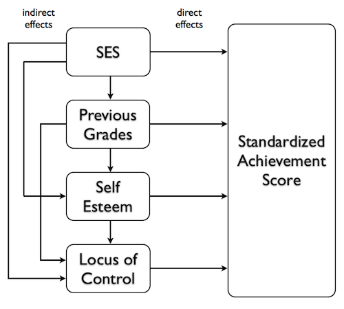
In the little regression universe that we've created for ourselves, the
predictors can influence the response potentially over several pathways. For
example, SES can have a direct effect on achievement scores, indicated by the
arrow that goes straight to the response, but it can also have effects that
follow indirect pathways. It can have an effect on locus of control, which
then affects achievement scores. It can have an effect on self esteem, which
can then act directly on achievement scores, but can also act through locus
of control. Following the other arrows around (other than the arrows showing
direct effects) will show us how WE THINK each of these predictors might have
an indirect effect on achievement scores.
Standard regression reveals only the direct effects of each predictor.
Because SES is treated as if it is entered last in a standard regression, all
of the indirect effects of SES have already been pruned away, having been
handed over to one of the other predictors, before SES gets to attempt to
claim variability in the response. Thus, SES is left only with its direct
pathway.
However, if SES were entered alone into a regression analysis (as
the only predictor, that is), we would get to see its total effect on
achievement score, which is its effect through both direct and indirect
pathways, because it wouldn't be competing with the other predictors for
response variability.
That's what a hierarchical regression does. If SES were entered first into
a hierarchical regression, it would get to claim all the response variability
it could without having to compete with the other predictors. In other words,
we wouldn't be seeing just the direct effect of SES on achievement scores, we'd
be seeing the total effect. Then when we enter Previous Grades second, we'd
get to see its total effect, provided none of that effect goes through SES and,
therefore, has already been claimed. Then we enter Self Esteem third, and we
see it's total effect, provided none of that goes through either Previous
Grades or SES. And so on.
In other words, standard regression reveals direct effects only. Hierarchical
regression reveals total effects, provided we have entered the predictors in
the correct order. And that is a BIG provided! Order of entering
the predictors is the biggest catch in hierarchical regression. How do we know
what order to use? Keith recommends drawing a diagram like the one above. Such
a diagram should make it clear in what order the variables should be entered.
If you can't draw such a diagram, then you probably shouldn't be using
hierarchical regression.
Note: I have to admit that it helped me a lot to have already written the
tutorial on Simple Mediation Analysis when I was
attempting to understand this!
Now For The Hierarchical Regression
Here are the hierarchical (or sequential as Keith calls it) multiple
regression results (Figure 5.3, page 79) as SPSS (I assume) calculated them.
The variables were entered one at a time in the order shown in the table.
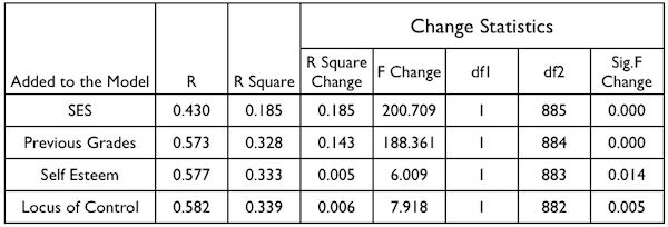
We already have some of these results. We need to recall the total sum of
squares, 86217.92, and we need to recall the ANOVA table we produced earlier.
> print(anova(lm.out), digits=7)
Analysis of Variance Table

Response: std.achieve.score
                  Df   Sum Sq   Mean Sq   F value     Pr(>F)
SES                1 15938.64 15938.645 246.49535 < 2.22e-16 ***
prev.grades        1 12344.62 12344.616 190.91274 < 2.22e-16 ***
self.esteem        1   391.62   391.623   6.05655  0.0140453 *
locus.of.control   1   512.00   512.001   7.91823  0.0050028 **
Residuals        882 57031.03    64.661
We can get the change in R-squared values by dividing each SS by the total.
> c(15938.64, 12344.62, 391.62, 512.00) / 86217.92
[1] 0.184864585 0.143179283 0.004542211 0.005938441
Of course, the R Square column is just the cumulative sum of those.
> cumsum(c(15938.64, 12344.62, 391.62, 512.00) / 86217.92)
[1] 0.1848646 0.3280439 0.3325861 0.3385245
And if you want to be really anal about it, the R column is the square root
of that.
> sqrt(cumsum(c(15938.64, 12344.62, 391.62, 512.00) / 86217.92))
[1] 0.4299588 0.5727511 0.5767028 0.5818286
Notice that our ANOVA table does not give the same tests, however (except for
the last one). Why? The answer is that the ANOVA table tests are done with a common
error term, namely, the one shown in the table. The tests in the SPSS table
can be obtained from the ANOVA for any term by pooling all the terms below it
in the table with the error term. For example, the test for prev.grades would be:
> ((12344.62)/1) / ((391.62+512.00+57031.03)/(1+1+882))    # F value
[1] 188.3613
> pf(188.3613, 1, 884, lower=F)                            # p-value
[1] 5.310257e-39
We could also do that like this, but ONLY the prev.grades test is available
in this output.
> anova(lm(std.achieve.score ~ SES + prev.grades, data=grades2))
Analysis of Variance Table

Response: std.achieve.score
             Df Sum Sq Mean Sq F value    Pr(>F)
SES           1  15939 15938.6  243.20 < 2.2e-16 ***
prev.grades   1  12345 12344.6  188.36 < 2.2e-16 ***
Residuals   884  57935    65.5
---
Signif. codes:  0 '***' 0.001 '**' 0.01 '*' 0.05 '.' 0.1 ' ' 1
Which tests are correct, the tests in R's ANOVA table, or the tests in the
SPSS table?
What Is The Correct Error Term?
According to every textbook I've ever read, and that's at least a couple,
the SPSS tests are correct. This is not a trivial point, because there are
multiple forums and R blogs online that advise doing a hierarchical regression
like this.
> model1 = lm(std.achieve.score ~ 1, data=grades2)
> model2 = lm(std.achieve.score ~ SES, data=grades2)
> model3 = lm(std.achieve.score ~ SES + prev.grades, data=grades2)
> model4 = lm(std.achieve.score ~ SES + prev.grades + self.esteem, data=grades2)
> anova(model1, model2, model3, model4, lm.out)
Analysis of Variance Table

Model 1: std.achieve.score ~ 1
Model 2: std.achieve.score ~ SES
Model 3: std.achieve.score ~ SES + prev.grades
Model 4: std.achieve.score ~ SES + prev.grades + self.esteem
Model 5: std.achieve.score ~ SES + prev.grades + self.esteem + locus.of.control
  Res.Df   RSS Df Sum of Sq        F    Pr(>F)
1    886 86218
2    885 70279  1   15938.6 246.4953 < 2.2e-16 ***
3    884 57935  1   12344.6 190.9127 < 2.2e-16 ***
4    883 57543  1     391.6   6.0566  0.014045 *
5    882 57031  1     512.0   7.9182  0.005003 **
---
Signif. codes:  0 '***' 0.001 '**' 0.01 '*' 0.05 '.' 0.1 ' ' 1
Notice that this exactly duplicates the results that are in the ANOVA table and
not those in the SPSS table. To duplicate the results that are in the SPSS
table, you would have to make these model comparisons two models at a time.
For example...
> anova(model2, model3)
Analysis of Variance Table

Model 1: std.achieve.score ~ SES
Model 2: std.achieve.score ~ SES + prev.grades
  Res.Df   RSS Df Sum of Sq      F    Pr(>F)
1    885 70279
2    884 57935  1     12345 188.36 < 2.2e-16 ***
---
Signif. codes:  0 '***' 0.001 '**' 0.01 '*' 0.05 '.' 0.1 ' ' 1
...would give the correct test for prev.grades. Or just...
> anova(model3) # not shown
...for the prev.grades test ONLY. So who says SPSS is right? Well, pretty
much everybody! The formula given for comparing two nested regression
analyses in every textbook I've consulted is this one, where for some
unaccountable reason L stands for the full model and S the reduced model.
(Maybe it means "larger" and "smaller." Didn't think of that!)
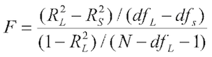
That this is the equivalent of the SPSS tests is easily demonstrated. To
test the effect of adding self.esteem to the model, for example, we would need
to know that the change in R-squared was .0045422, that the change in df was 1,
that R-squared for the full model, including self.esteem, was .33259, and N
was 887, after dropping all the cases with missing values. So...
> .0045422/((1-.33259)/(887-3-1))  # F-value
[1] 6.009443
Since there is no function in R that automates a hierarchical regression, the
lesson here is BE CAREFUL WITH THE ERROR TERM.
Entering Variables In Blocks
Variables don't have to be entered one at a time into a hierarchical
regression. They can also be entered in blocks. This might happen, for example,
if the researcher wanted to enter all psychological variables at one time, or
if the researcher was uncertain about the order in which they should be entered.
Let's say in the current example we wanted to enter self.esteem and
locus.of.control at the same time. (Frankly, I was unconvinced by Keith's
argument concerning the order in which these variables should be entered.)
The increase in R-squared can be obtained by summing the SSes in the ANOVA
table and dividing by the total SS.
> (391.62 + 512.00) / 86217.92
[1] 0.01048065
Which is just the sum of the individual increases in R-squared. The test on
this would be the following.
> anova(model3, lm.out)
Analysis of Variance Table

Model 1: std.achieve.score ~ SES + prev.grades
Model 2: std.achieve.score ~ SES + prev.grades + self.esteem + locus.of.control
  Res.Df   RSS Df Sum of Sq      F    Pr(>F)
1    884 57935
2    882 57031  2    903.62 6.9874 0.0009754 ***
---
Signif. codes:  0 '***' 0.001 '**' 0.01 '*' 0.05 '.' 0.1 ' ' 1
Model 3 was the model before this block of variables was entered, i.e., the
model that included SES and prev.grades, and lm.out was the model after this
block of variables was entered. This is in agreement with the SPSS output that
is in Figure 5.9 in Keith. So, good, SPSS got it right again!
Question
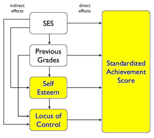
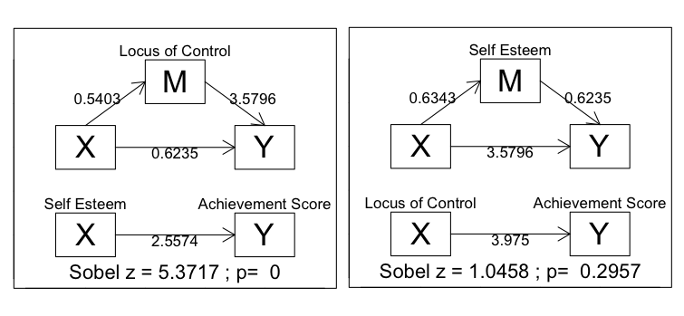
I couldn't help noticing how much the shaded portion of the NELS diagram at
left resembles a Simple Mediation Analysis, or
rather, the diagram one would draw to represent such an analysis. As I said
above, I'm not convinced Keith got self.esteem and locus.of.control in the
correct order in the hierarchical regression. I believe the order should be
reversed. I believe locus.of.control, being something that is learned from
your environment, is the causally prior (or at least more important) variable.
(Not being an expert on either of these constructs, I doubt that my "belief"
should carry much weight, and I'm just playing devil's advocate!) So the
mediation analysis people should
forgive me, but I decided to play a little fast and loose with a mediation
analysis. My "hypothesis" (such as it is) is that, if locus of control is
entered as the mediator, it will completely sap self-esteem of its effect on
achievement scores (complete mediation), because it's locus of control that's
having the effect on scores and not self-esteem. That relationship would not
be seen in the hierarchical regression as we've done it, because by the time
locus of control got into the model, self-esteem has already grabbed a large
(and undeserved) piece of the pie. Locus of control has been short circuited,
so to speak. On the other hand, if the roles of self-esteem
and locus of control were reversed in the mediation analysis, i.e., self-esteem
entered as the mediator, we'd see virtually no mediation. I did those two
analyses using the mediate() function that is
discussed in the mediation analysis tutorial. The results are in the following
diagrams (created by that function). The numbers on the lines are regression
coefficients from the various models used to do the mediation analysis (see
that tutorial).
 For the record, these were the commands used. The
mediate() function is in the tutdata folder that you may have
downloaded to accompany these tutorials.
For the record, these were the commands used. The
mediate() function is in the tutdata folder that you may have
downloaded to accompany these tutorials.
> with(grades2, mediate(self.esteem, std.achieve.score, locus.of.control,
+    names=c("Self Esteem","Achievement Score","Locus of Control")))
       a        b        c       cp  sobel.z        p
0.540276 3.579580 2.557419 0.623457 5.371740 0.000000
> with(grades2, mediate(locus.of.control, std.achieve.score, self.esteem,
+    names=c("Locus of Control","Achievement Score","Self Esteem")))
       a        b        c       cp  sobel.z        p
0.634315 0.623457 3.975048 3.579580 1.045782 0.295662
It appears my "hypothesis" was confirmed. Pretty close anyway. My question
is, what does it mean? Does it mean I'm right and these variables
were entered in the wrong order in the hierarchical regression? Does it
mean the opposite? Or do the two analyses bear no relationship to one
another?
I don't know the answers to these questions, and I suspect they are not to
be found in the above analyses. That's why we are constantly warned that
techniques like these (hierarchical regression, mediation analysis, path
analysis) are not useful for exploratory analyses. These are correlational
data, and as we know, we can twist correlational data around our little
fingers and make them do just about anything we want. Also, there is no
guarantee that these are the only variables, or even the most important
variables, that we should be looking at.
This is one case where the hard work should definitely come BEFORE the
analysis. It's up to us to be familiar enough with the phenomena under
investigation that we can form reasonable and rational theories of causation.
We CANNOT get those from correlational data. Correlational data can be
consistent or inconsistent with our previously formed theories, but that's
all. There is a much quoted warning (concerning path analysis, but equally
applicable to any of these similar techniques) from Everitt and Dunn (1991)
that is worth repeating here: "However convincing, respectable and reasonable
a path diagram... may appear, any causal inferences extracted are rarely more
than a form of statistical fantasy."
- Everitt, B. S. and Dunn, G. (1991). Applied multivariate data analysis.
London: Edward Arnold.
created 2016 March 29
| Table of Contents
| Function Reference
| Function Finder
| R Project |
|