
| Table of Contents
| Function Reference
| Function Finder
| R Project |
CHI SQUARE TEST OF INDEPENDENCE
Syntax
From the help page, the syntax of the chisq.test()
function is...
chisq.test(x, y = NULL, correct = TRUE,
           p = rep(1/length(x), length(x)), rescale.p = FALSE,
           simulate.p.value = FALSE, B = 2000)
This function is used for both the goodness of fit test and the test of
independence, and which test it does depends upon what kind of data you feed
it. If "x" is a numeric vector or a one-dimensional table of numerical
values, a goodness of fit test will be done (or attempted), treating "x" as a
vector of observed frequencies. If "x" is a 2-D table, array, or matrix, then
it is assumed to be a contingency table of frequencies, and a test of
independence will be done.
Ignore "y". (See below for when to use y.) The "correct=TRUE" option
applies the Yates continuity correction when "x" is a 2x2 table. Set this to
FALSE if the correction is not desired. For the goodness of fit test, set "p"
equal to the null hypothesized proportions or probabilies for each of the
categories represented in the vector "x". These must add exactly to 1.
For the test of independence, the p= option is irrelevant, as the expected
frequencies are calculated from the observed frequencies, x.
Textbook Problems
The following textbook-like problem uses data from Hand et al. (1994).
       Senie et al. (1981) investigated the relationship between age and
       frequency of breast self-examination in a sample of women (Senie,
       R. T., Rosen, P. P., Lesser, M. L., and Kinne, D. W. Breast self-
       examinations and medical examination relating to breast cancer
       stage. American Journal of Public Health, 71, 583-590.)
       A summary of the results is presented in the following table:

                    Frequency of breast self-examination
                    ------------------------------------
       Age          Monthly      Occasionally      Never
       -------------------------------------------------
       under 45         91            90             51
       45 - 59         150           200            155
       60 and over     109           198            172
       ------------------------------------------------
       From Hand et al., page 307, table 368.
The data have already been tabled for us in most textbook problems. We just have
to get the data into an R data object. There are several ways to do this.
> row1 = c(91,90,51)                   # or col1 = c(91,150,109)
> row2 = c(150,200,155)                # and col2 = c(90,200,198)
> row3 = c(109,198,172)                # and col3 = c(51,155,172)
> data.table = rbind(row1,row2,row3)   # and data.table = cbind(col1,col2,col3)
> data.table
     [,1] [,2] [,3]
row1   91   90   51
row2  150  200  155
row3  109  198  172
> chisq.test(data.table)

        Pearson's Chi-squared test

data:  data.table
X-squared = 25.086, df = 4, p-value = 4.835e-05
If the data are available in an electronic document, like this one, it can be
entered into R using the scan() function.
> ls()
[1] "data.table" "row1"       "row2"       "row3"
> rm(list=ls())                             # Clean up a bit first!
> the.data = scan()
1:   91            90             51
4:  150           200            155
7:  109           198            172
10:
Read 9 items
> the.data                                  # scan produces a vector
[1]  91  90  51 150 200 155 109 198 172
> data.matrix = matrix(the.data, byrow=T, nrow=3)
> data.matrix                               # which we convert to a matrix
     [,1] [,2] [,3]
[1,]   91   90   51
[2,]  150  200  155
[3,]  109  198  172
> chisq.test(data.matrix)$statistic         # keeping the output brief
X-squared
 25.08597
The data table can be copied and pasted one row at a time into the
scan()
function. The result will be a vector in which the data are entered row-wise.
A matrix is then created using the matrix()
function, which expects the
data vector to contain column-wise data, i.e., 91, 150, 109, 90, ..., 172. This
behavior can be changed with the "byrow=T" option. The "nrow=" option specifies
how many rows to create in the matrix.
If the problem asks for further data summarization, you will probably want
to give names to the rows and columns of the data table first, since this will
make R output easier to read and especially make barplots much easier to
construct.
> dimnames(data.matrix) = list(Age=c("lt.45",45.to.59","ge.60"),
Error: unexpected symbol in "dimnames(data.matrix) = list(Age=c("lt.45",45.to.59"
And here, in all fairness to those who would prefer a hunt-and-click interface,
I suppose I should interpose a comment. This error drove me nuts for a good ten
minutes or more. It even prompted me to go back and look at a previous tutorial
on data entry. To use a command line interface, you do have to have an eye for
minutiae. Do you see the mistake? It took me awhile to spot it! I left out an
open quote. The tip off should have been that R stopped outputting the error
message at the closed quote that had no matching open quote. Let's see if I can
get it right this time. (The old days! I was a relative newbie then. After years
of R-ing, I know what to look for now. I would have spotted that missing quote
in a twinkling. That's my story and I'm sticking to it!)
> dimnames(data.matrix) = list(Age=c("lt.45","45.to.59","ge.60"),
+                              Freq=c("Monthly","Occasionally","Never"))
> data.matrix
          Freq
Age        Monthly Occasionally Never
  lt.45         91           90    51
  45.to.59     150          200   155
  ge.60        109          198   172
> ### At last!
> ### Examine marginal distributions...
> addmargins(data.matrix)
          Freq
Age        Monthly Occasionally Never  Sum
  lt.45         91           90    51  232
  45.to.59     150          200   155  505
  ge.60        109          198   172  479
  Sum          350          488   378 1216
> ### Examine conditional distributions...
> prop.table(data.matrix, 1)                # relative to margin 1, the row margin
          Freq
Age          Monthly Occasionally     Never
  lt.45    0.3922414    0.3879310 0.2198276
  45.to.59 0.2970297    0.3960396 0.3069307
  ge.60    0.2275574    0.4133612 0.3590814
> ### And finally a barplot...
> barplot(data.matrix, beside=T)           # output not shown
> ### Okay, a better barplot... (you could type this into a script window)
> barplot(t(data.matrix), beside=T, legend=T, ylim=c(0,250),         # t() for transpose
+         ylab="Observed frequencies in sample",
+         main="Frequency of Breast Self-Examination by Age")
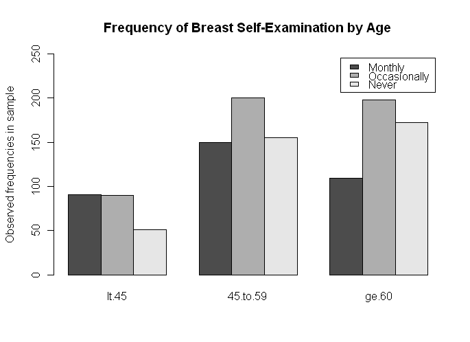 In a future tutorial, we'll learn how to move the legend to a more appealing
location on the graph.
In a future tutorial, we'll learn how to move the legend to a more appealing
location on the graph.
Data From a Table Object
You may remember the following data object, which was used in a couple
previous tutorials.
> UCBAdmissions                                  # output not shown
> ftable(UCBAdmissions, row.vars=c("Admit"))     # a more compact version
         Gender Male                     Female
         Dept      A   B   C   D   E   F      A   B   C   D   E   F
Admit
Admitted         512 353 120 138  53  22     89  17 202 131  94  24
Rejected         313 207 205 279 138 351     19   8 391 244 299 317
> round(prop.table(ftable(UCBAdmissions, row.vars=c("Admit")),2),2)
         Gender Male                          Female
         Dept      A    B    C    D    E    F      A    B    C    D    E    F
Admit
Admitted        0.62 0.63 0.37 0.33 0.28 0.06   0.82 0.68 0.34 0.35 0.24 0.07
Rejected        0.38 0.37 0.63 0.67 0.72 0.94   0.18 0.32 0.66 0.65 0.76 0.93
And don't think for a moment it didn't take me a little trial and error to get
the last version of the data table!
Suppose we want a chi square test of Admit by Gender in Dept. B only. I'll
begin by extracting just those data (although that is technically
unnecessary).
> deptB = UCBAdmissions[,,2]           # all rows, all cols, but only of layer 2
> deptB
          Gender
Admit      Male Female
  Admitted  353     17
  Rejected  207      8
> chisq.test(deptB)

        Pearson's Chi-squared test with Yates' continuity correction

data:  deptB
X-squared = 0.0851, df = 1, p-value = 0.7705

> chisq.test(deptB)$expected
          Gender
Admit          Male    Female
  Admitted 354.1880 15.811966
  Rejected 205.8120  9.188034
No significant relationship is found between Admit and Gender in Dept. B, as
might have been expected from examination of the data table. I also took a look
at the expected frequencies, just because I could, although it's not so crucial
to do so when the null hypothesis is retained. Notice that Yate's correction for
continuity is applied by default when a 2x2 table is entered into the chi square
procedure. This behavior can be turned off with the option "correct=F".
> chisq.test(deptB, correct=F)

        Pearson's Chi-squared test

data:  deptB
X-squared = 0.2537, df = 1, p-value = 0.6145
Data From a Data Frame
The data frame "survey" in the "MASS" package contains responses from 237
statistics students to a series of questions, some of which resulted in
categorical answers. For one item, the students were asked to fold their arms,
and the recorded result was which arm was on top: right, left, or neither. Let's
see how this variable relates to the sex of the student.
> data(survey, package="MASS")
> attach(survey)
> table(Sex, Fold)
        Fold
Sex      L on R Neither R on L
  Female     48       6     64
  Male       50      12     56
In this case, the two vectors of interest, "Sex" and "Fold", both contain
categorical values on a case by case basis. You could table them first (as we
just did), store this table in a data object, and enter the name of this
data object into the chisq.test() function, but
in cases like these, R allows a simpler syntax.
> chisq.test(x=Sex, y=Fold)            # simply chisq.test(Sex, Fold) will do

        Pearson's Chi-squared test

data:  Sex and Fold
X-squared = 2.5741, df = 2, p-value = 0.2761
As long as the two data vectors, X and Y, are categorical, and they are
arranged such that Xi corresponds on a case by case basis to
Yi, you need only to enter the names of the two data vectors
into the chi square test function. R will do the implied crosstabulation for
you.
> detach(survey) # Don't forget!
Alternatives When the EFs Are Small
The following data are from a Stanford University study of the effectiveness
of the antidepressant Celexa in the treatment of compulsive shopping. These data
were found in Verzani (2005, p.262f), and the analysis here is similar to his.
                     outcome
                 -----------------
       treat     worse same better
       ---------------------------
       Celexa      2     3     7
       placebo     2     8     2
       ---------------------------

> freqs = c(2, 2, 3, 8, 7, 2)               # entered "down the columns" this time
> data.matrix = matrix(freqs, nrow=2)       # fills down columns by default
> dimnames(data.matrix) = list(treatment=c("Celexa","placebo"),
+                              outcome=c("worse","same","better"))
> data.matrix
         outcome
treatment worse same better
  Celexa      2    3      7
  placebo     2    8      2

> chisq.test(data.matrix)

        Pearson's Chi-squared test

data:  data.matrix
X-squared = 5.0505, df = 2, p-value = 0.08004

Warning message:
In chisq.test(data.matrix) : Chi-squared approximation may be incorrect

> chisq.test(data.matrix)$expected
         outcome
treatment worse same better
  Celexa      2  5.5    4.5
  placebo     2  5.5    4.5
Warning message:
In chisq.test(data.matrix) : Chi-squared approximation may be incorrect
The chi square procedure produces a warning message (somewhat cryptic) when any
of the expected frequencies fall below 5. In this case, most of them do, which
should lead us to be concerned about the accuracy of any p-value calculated
from the chi-squared distribution. Since the p-value is close to .05, we might
want to try a more accurate method. What can we do?
There are two choices: a Fisher Exact Test, and a p-value calculated by
Monte Carlo simulation. Let's look at the Fisher Exact Test first.
You may be thinking, "Um, doesn't the Fisher Exact Test work only for 2x2
tables?" Yes, and when a 2x2 table is supplied, R will give you the exact
p-value calculated from the hypergeometric distribution. However, in R, the
Fisher Exact Test has been extended to work with larger tables, provided the
obtained frequencies are not too large. You should see the help page for the
details of how this has been done.
> fisher.test(data.matrix)

        Fisher's Exact Test for Count Data

data:  data.matrix
p-value = 0.07303
alternative hypothesis: two.sided
The Fisher Exact Test suggests that the chi square procedure gave us a fairly
accurate result in spite of the low expected frequencies. And don't get your
feathers in a ruffle here, because although there is an "alternative=" option
for this test, it works ONLY for 2x2 tables, in which case R calculates and
tests the odds ratio for significance. You might want to investigate the Fisher
Exact Test further on your own, as there is additional output when a 2x2 table
is supplied.
The other alternative is to simulate the sampling distribution of the test
statistic (in this case, chi squared) using Monte Carlo methods. (To find out
more about this, read the Resampling Techniques
tutorial.) Fortunately, the chisq.test() function
incorporates an option that automates this complex procedure for us.
> chisq.test(data.matrix, simulate.p.value=T, B=999)

        Pearson's Chi-squared test with simulated p-value (based on 999
        replicates)

data:  data.matrix
X-squared = 5.0505, df = NA, p-value = 0.111
The "simulate.p.value=T" option (default value is FALSE) does the Monte Carlo
simulation using "B=999" (default value is B=2000) replicates. It doesn't look
like we can fish up a signficant relationship here!
revised 2016 January 27
| Table of Contents
| Function Reference
| Function Finder
| R Project |
|