
| Table of Contents
| Function Reference
| Function Finder
| R Project |
ONEWAY BETWEEN SUBJECTS ANOVA
Assumptions of Analysis of Variance
Traditional parametric analysis of variance makes the following assumptions:
- Random sampling, or at the very least, random assignment to groups.
- Independence of scores on the response variable -- i.e., what you get
from one subject should be in no way influenced by what you get from
any of the others.
- Sampling from normal populations within each cell of the design.
- Homogeneity of variance -- the populations within each cell of the
design should all have the same variance.
The first two of these are methodological issues and will not be discussed
further. The last two are assumptions we need to look at statistically.
A brief note: I very much prefer the title "between groups anova" for these
techniques, because the effect is going to show up between (among) group means
and not between subjects. I have occasionally seen that appellation used,
but "between subjects" is the more common one, so I defer to the majority.
Oneway ANOVA
R supplies a variety of ways of doing analysis of variance, but among the
simpliest is to use the oneway.test() function for
simple between subjects designs (only). There are advantages and disadvantages
to using this function, as will be pointed out. First, let's get some data.
> data(InsectSprays)
> str(InsectSprays)
'data.frame':   72 obs. of  2 variables:
 $ count: num  10 7 20 14 14 12 10 23 17 20 ...
 $ spray: Factor w/ 6 levels "A","B","C","D",..: 1 1 1 1 1 1 1 1 1 1 ...
 > summary(InsectSprays)
     count       spray
 Min.   : 0.00   A:12
 1st Qu.: 3.00   B:12
 Median : 7.00   C:12
 Mean   : 9.50   D:12
 3rd Qu.:14.25   E:12
 Max.   :26.00   F:12
The data are from an agricultural experiment in which six different insect
sprays were tested in many different fields, and the response variable (DV) was
a count of insects found in each field after spraying. Let's have a closer look.
> attach(InsectSprays)
> tapply(count, spray, mean)
        A         B         C         D         E         F
14.500000 15.333333  2.083333  4.916667  3.500000 16.666667
> tapply(count, spray, var)
        A         B         C         D         E         F
22.272727 18.242424  3.901515  6.265152  3.000000 38.606061
> tapply(count, spray, length)              # okay, as there are no missing values
 A  B  C  D  E  F
12 12 12 12 12 12
There are large differences in the means, but there are also large differences
in the variances (and worse yet, the means and variances appear to be related).
At least the design is balanced. Boxplots are a good way to present the data
graphically.
> boxplot(count ~ spray) # boxplot(count~spray, data=InsectSprays) if not attached
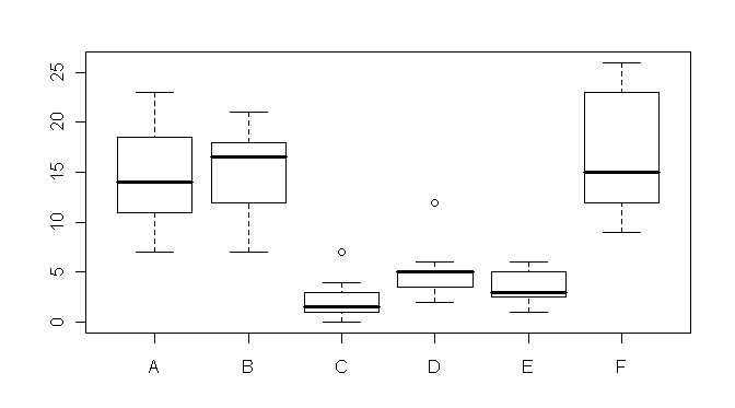 Wow! It hurts my eyes just to look at it! The distributions are skewed, there
are outliers, and homogeneity is out the window! Nevertheless, we shall proceed
naively, just to demonstrate how the
oneway.test() function works. It's quite simple.
The syntax is...
Wow! It hurts my eyes just to look at it! The distributions are skewed, there
are outliers, and homogeneity is out the window! Nevertheless, we shall proceed
naively, just to demonstrate how the
oneway.test() function works. It's quite simple.
The syntax is...
oneway.test(formula, data, subset, na.action, var.equal = FALSE)
...and so we run our test as follows.
> oneway.test(count ~ spray)      # oneway.test(count~spray, data=InsectSprays) if not attached

        One-way analysis of means (not assuming equal variances)

data:  count and spray
F = 36.0654, num df = 5.000, denom df = 30.043, p-value = 8e-12
By default, oneway.test() applies a Welch-like
correction for
nonhomogeneity, so this is not the answer your intro stat students would have
gotten if they were doing the problem by hand. If you want to turn off this
behavior, set the "var.equal=" option to TRUE. Another caution: The function
demands a formula interface, so the data should be in a proper data frame and
not in vectors group by group. (But see a further comment on this below.) There
is a "data=" option if you don't care to attach the data frame. One more
thing...
> detach(InsectSprays)
> ifelse(InsectSprays$count==26, NA, InsectSprays$count)
 [1] 10  7 20 14 14 12 10 23 17 20 14 13 11 17 21 11 16 14 17 17 19 21  7 13  0
[26]  1  7  2  3  1  2  1  3  0  1  4  3  5 12  6  4  3  5  5  5  5  2  4  3  5
[51]  3  5  3  6  1  1  3  2  6  4 11  9 15 22 15 16 13 10 NA NA 24 13
> ifelse(InsectSprays$count==26, NA, InsectSprays$count) -> new.data      # with missing values
> InsectSprays$sprays -> sprays        # put the IV vector in the workspace for demo purposes
> ls()
[1] "InsectSprays" "new.data"     "sprays"
> oneway.test(new.data ~ sprays)

        One-way analysis of means (not assuming equal variances)

data:  new.data and sprays
F = 35.5121, num df = 5.000, denom df = 28.697, p-value = 1.926e-11

> oneway.test(new.data ~ sprays, var.equal=T)    # assuming homogeneity of variance

	One-way analysis of means

data:  new.data and sprays
F = 36.8048, num df = 5, denom df = 64, p-value < 2.2e-16
The oneway.test() function is well behaved when
it comes to missing values because the default is to omit them from the analysis.
How do we know that? There doesn't seem to be any default set in the syntax. R
maintains a list of default options, one of which is "na.action". To see it, do
this.
> options("na.action")       # to see them all, and there are a lot, use options()
$na.action
[1] "na.omit"
This means you should
check your data for missing values before hand, as this procedure will not tell
you about them if they exist. We saw by using the
summary() function above that there were no NAs in the original data.
Now we have some, so we should think what to do about them. Setting the
"na.action=" option in the function will change its behavior towards NAs, and
to see the choices we have, we can do help(na.action).
Basically, the two alternatives are "na.omit" and "na.fail". The latter will
make the procedure fail if there are missing values. (I bet you guessed that!)
> oneway.test(new.data ~ sprays, na.action="na.fail")
Error in na.fail.default(list(new.data = c(10, 7, 20, 14, 14, 12, 10,  :
  missing values in object
Another thing you may have noticed--R does not require the vectors it is
working with in a formula to be in a data frame. They can be ordinary
vectors in the workspace, as long as one is a proper response variable vector,
and the other can be considered (coerced to) a factor. I.e., the procedure will
work as long as it has proper data-frame-like vectors to work with.
> ls()
[1] "InsectSprays" "new.data"     "sprays"
> rm(new.data, sprays)
Don't forget to clean up your mess.
Testing For Homogeneity of Variance
R incorporates the Bartlett test to test the null hypothesis of equal group
variances.
> bartlett.test(count ~ spray, data=InsectSprays)

        Bartlett test of homogeneity of variances

data:  count by spray
Bartlett's K-squared = 25.9598, df = 5, p-value = 9.085e-05
Busted! Another test implemented in the base packages is the Fligner-Killeen
(median) test. The help page says it works with a formula interface, but it
doesn't, so you have to send it x=DV and g=IV.
> fligner.test(x=InsectSprays$count, g=InsectSprays$spray)

	Fligner-Killeen test of homogeneity of variances

data:  InsectSprays$count and InsectSprays$spray
Fligner-Killeen:med chi-squared = 14.4828, df = 5, p-value = 0.01282
The Levene test, which has become more or less standard these days, is not
implemented in the base packages, but it is available in the optional package
"car", if you have that installed (see Package
Management). Be careful with the syntax, because it is annoyingly
different from the above tests (but more logical when it comes right down
to it). A formula interface will also work.
> library(car)               # this will generate an error if "car" has not been installed
> leveneTest(y=InsectSprays$count, group=InsectSprays$spray)
Levene's Test for Homogeneity of Variance (center = median)
      Df F value   Pr(>F)
group  5  3.8214 0.004223 **
      66
--- (# additional output deleted)
This is not actually the original Levene test. It is a median-centered
version of the Levene test,
which is supposedly more robust. The original can be obtained this way.
> leveneTest(y=InsectSprays$count, group=InsectSprays$spray, center=mean)
Levene's Test for Homogeneity of Variance (center = mean)
      Df F value    Pr(>F)
group  5  6.4554 6.104e-05 ***
      66
--- (# additional output deleted)
The null hypothesis for all these tests is that the variances are the same
(homogeneous). All the tests are rejecting that hypothesis.
The aov() Function
Syntax:
aov(formula, data = NULL, projections = FALSE, qr = TRUE,
    contrasts = NULL, ...)
The advantage of using the oneway.test()
function is obviously the Welch correction for nonhomogeneity. The disadvantages
are it doesn't give you a lot of information in the output, and there are no
post hoc tests readily available. The standard R function for all kinds of ANOVA
is aov(). It's best to store (assign)
the output of this function and then to extract the information you want
by way of various extractor functions. This is the way we will be working
from now on with all statistical procedures more complex than chi square
and the t-test. Here is an example using the InsectSprays data.
> aov.out = aov(count ~ spray, data=InsectSprays)
> summary(aov.out)
            Df  Sum Sq Mean Sq F value    Pr(>F)
spray        5 2668.83  533.77  34.702  <2.2e-16 ***
Residuals   66 1015.17   15.38
---
Signif. codes:  0 '***' 0.001 '**' 0.01 '*' 0.05 '.' 0.1 ' ' 1
This is the same result you would get from the
oneway.test() function but without the full ANOVA summary table and a few
other niceties.
> oneway.test(count ~ spray, data=InsectSprays, var.eq=T)

	One-way analysis of means

data:  count and spray
F = 34.7023, num df = 5, denom df = 66, p-value < 2.2e-16
The aov() function does not have the Welch
correction available, but it does give the full summary table. It also saves
a lot of information about the analysis. For example, at this point the
assumptions can be tested using graphical methods.
> par(mfrow=c(1,2))          # set graphics window to plot side-by-side
> plot(aov.out, 1)           # graphical test of homogeneity
> plot(aov.out, 2)           # graphical test of normality
> # close the graphics device to reset its parameters
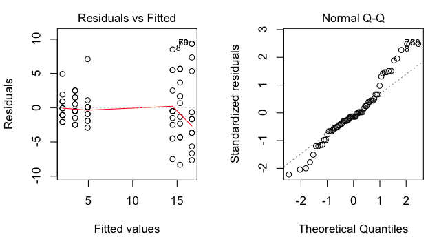 The graph on the left shows the residuals (score - group mean) clearly getting
larger as the group means get larger, a bad pattern, but not unusual when the
DV results from counting something. The graph on the right shows that the
residuals are not normally distributed, so the normality assumption is also
violated. (Note: A similar graphical test of residuals by groups can be had
this way, provided there are no missing values in the data:
The graph on the left shows the residuals (score - group mean) clearly getting
larger as the group means get larger, a bad pattern, but not unusual when the
DV results from counting something. The graph on the right shows that the
residuals are not normally distributed, so the normality assumption is also
violated. (Note: A similar graphical test of residuals by groups can be had
this way, provided there are no missing values in the data:
> boxplot(aov.out$resid ~ InsectSprays$spray)
If there are missing values, these two vectors will be of unequal lengths,
and this will fail. Also, this method does not allow the size of the
residuals to be seen in relation to the size of the group means.)
There is not much more to say about aov() at the
moment except that R calculates ANOVAs as special cases of linear models, so
much of what will eventually be said about the lm()
function applies. Another advantage of using aov()
will be seen in the next section.
A Post Hoc Test
The Tukey Honestly Significant Difference test has been implemented in the
R base distribution as the default post hoc test for ANOVA main effects. It's
easily enough applied once the output of aov()
has been stored in the workspace.
> TukeyHSD(aov.out)
  Tukey multiple comparisons of means
    95% family-wise confidence level

Fit: aov(formula = count ~ spray, data = InsectSprays)

$spray
           diff        lwr       upr     p adj
B-A   0.8333333  -3.866075  5.532742 0.9951810
C-A -12.4166667 -17.116075 -7.717258 0.0000000
D-A  -9.5833333 -14.282742 -4.883925 0.0000014
E-A -11.0000000 -15.699409 -6.300591 0.0000000
F-A   2.1666667  -2.532742  6.866075 0.7542147
C-B -13.2500000 -17.949409 -8.550591 0.0000000
D-B -10.4166667 -15.116075 -5.717258 0.0000002
E-B -11.8333333 -16.532742 -7.133925 0.0000000
F-B   1.3333333  -3.366075  6.032742 0.9603075
D-C   2.8333333  -1.866075  7.532742 0.4920707
E-C   1.4166667  -3.282742  6.116075 0.9488669
F-C  14.5833333   9.883925 19.282742 0.0000000
E-D  -1.4166667  -6.116075  3.282742 0.9488669
F-D  11.7500000   7.050591 16.449409 0.0000000
F-E  13.1666667   8.467258 17.866075 0.0000000
The procedure prints out the difference between means for each pair of groups,
the lower and upper limits of a 95% confidence interval for that difference
(change this by setting the "conf.level=" option), and the p-value for the
Tukey test. Of course, the validity of all of this depends upon how well we
have satisfied the assumptions of the ANOVA test in the first place, but
with p-values as low as ones we are seeing here, I'm betting these results
are pretty robust.
There is more on post hoc tests in the
Multiple Comparisons tutorial.
Power
The syntax of the power.anova.test()
function is...
power.anova.test(groups = NULL, n = NULL,
                 between.var = NULL, within.var = NULL,
                 sig.level = 0.05, power = NULL)
Exactly one of those options should be left at NULL, and it will be calculated
from the others. However, you should be aware that "between.var=" and
"within.var=" do not refer to variances, i.e., mean squares. The value of
"between.var=" should be set to the anticipated variance of the group means.
(MS-between would be n-per-group times the variance of the group means, so
variance of the group means is MS-between/n-per-group.) I'm
not clear on how the "within.var=" option should be set (and don't bother going
to the help page for help!), but I BELIEVE it is the anticipated MS-error,
which is to say the per group standard deviation squared. It's not necessary
actually to have values for these but only the anticipated ratio of them. For
example, the following example occurs on the help page.
power.anova.test(groups=4, between.var=1, within.var=3,
                 power=.80)
# n = 11.92613
The following example occurs online at
Dr. Steve Thompson's website, and leads me to believe I am correct.
> attach(InsectSprays)
> meancounts = tapply(count, spray, mean)
> var(meancounts)
[1] 44.48056
> summary(aov(count ~ spray))
            Df  Sum Sq Mean Sq F value    Pr(>F)
spray        5 2668.83  533.77  34.702 < 2.2e-16 ***
Residuals   66 1015.17   15.38
---
Signif. codes:  0 '***' 0.001 '**' 0.01 '*' 0.05 '.' 0.1 ' ' 1

> power.anova.test(groups=6, between.var=44.48, within.var=15.38, power=.9)

     Balanced one-way analysis of variance power calculation

         groups = 6
              n = 2.28168
    between.var = 44.48
     within.var = 15.38
      sig.level = 0.05
          power = 0.9

 NOTE: n is number in each group

> detach(InsectSprays)
> rm(meancounts)
This is just one example where the R help pages really fall down on the job, but
R is becoming popular enough that an answer can usually be found online, if you
are willing to look.
Once again I have to warn about using the power functions after the fact
(post hoc power). The functions are meant to be used during the design phase
of the experiment, before data are collected. See Howell's excellent textbook,
Statistical Methods for Psychology, for a discussion of this.
An Alternative to the Oneway Test
When assumptions fail, a nonparametric test is often our refuge. In
cases like this, the Kruskal-Wallis oneway ANOVA is often recommended.
> kruskal.test(count ~ spray, data=InsectSprays)

        Kruskal-Wallis rank sum test

data:  count by spray
Kruskal-Wallis chi-squared = 54.6913, df = 5, p-value = 1.511e-10
However, the Kruskal-Wallis test should not be regarded as a panacea. It is
primarily intended to cure problems with normality. It performs best when the
distributions all have the same shape, and when there is homogeneity of
variance.
Bootstrap
A bootstrap solution to this problem suggests the F* critical value at alpha
= .05 should be set closer to 2.79 than to the theoretical value of 2.35
that comes from the F(5,66)-distribution. This is discussed in the tutorial on
Resampling Techniques.
Treatment Contrasts
This material has been moved to a new tutorial on
Multiple Comparisons.
revised 2016 January 31
| Table of Contents
| Function Reference
| Function Finder
| R Project |
|