
| Table of Contents
| Function Reference
| Function Finder
| R Project |
SINGLE SAMPLE t TEST
Syntax
The syntax for the t.test() function is given
here from the help page in R.
## Default S3 method:
t.test(x, y = NULL,
       alternative = c("two.sided", "less", "greater"),
       mu = 0, paired = FALSE, var.equal = FALSE,
       conf.level = 0.95, ...)

## S3 method for class 'formula':
t.test(formula, data, subset, na.action, ...)
"S3" refers to the S language (version 3), which is often the same as the
methods and syntax used by R. In the case of the
t.test() function, there
are two alternative syntaxes, the default, and the "formula" syntax. The
formula syntax will be discussed in the following two tutorials on the
two-sample t-tests. The default syntax requires a data vector, "x", to be
specified. The "alternative=" option is set by default to "two.sided" but can
be set to any of the three values shown above. The default null hypothesis is
"mu = 0", which should be changed by the user if this is not your null
hypothesis. The rest is either irrelevant to this tutorial or can be ignored
for the moment.
Hey! What Happened to the z Test?
The z-tests have not been implimented in the default R packages, although
they have been included in an optional, add-on library called "UsingR." (See
the Package Management tutorial for details on how
to add this library to R.)
The t Test With a Single Sample
What is normal human body temperature (taken orally)? We've all been taught
since grade school that it's 98.6 degrees Fahrenheit, and never mind that
what's normal for one person may not be "normal" for another! So from a
statistical point of view, we should abandon the word "normal" and confine
ourselves to talking about average human body temperature. We hypothesize that
mean human body temperature is 98.6 degrees, because that's what we were told
in the third grade. The data set "Normal Body Temperature, Gender, and Heart
Rate" bears on this hypothesis. It is not built-in, so we will have to enter
the data. The data are from a random sample (supposedly) of 130 cases and has
been posted at the Journal of Statistical Education's data
archive. The original source of the data is Mackowiak, P. A., Wasserman,
S. S., and Levine, M. M. (1992). A Critical Appraisal of 98.6 Degrees F, the
Upper Limit of the Normal Body Temperature, and Other Legacies of Carl Reinhold
August Wunderlich. Journal of the American Medical Association,
268, 1578-1580. Direct your browser here to see the data:
normtemp.txt.
There are several ways you can try to get the data into R. I will go through
them one at a time. The first and most straightforward one is to read it in
directly from the linked webpage above. The data are in tabular format (data
values separated by white space), and there are no column headers. (Note: In
the following R commands, header=F is actually unnecessary, because that's the
default for the read.table() function.)
> file = "http://ww2.coastal.edu/kingw/statistics/R-tutorials/text/normtemp.txt"
> normtemp = read.table(file, header=F, col.names=c("temp","sex","hr"))
> head(normtemp)
  temp sex hr
1 96.3   1 70
2 96.7   1 71
3 96.9   1 74
4 97.0   1 80
5 97.1   1 73
6 97.1   1 75
Another way is to download that page using your browser. Right click on it, pick
Save Page As...,
and then save it wherever you save downloads, probably your Downloads folder.
Move it from that location to your working directory (Rspace, if that's where
you do your R work), and then load it from there. (Note: This only works because
the page is pure text and contains nothing but the data.)
> rm(normtemp)                         # if the last method worked for you
> normtemp = read.table(file = "normtemp.txt", header=F, col.names=c("Temp","Sex","HR"))
> head(normtemp)
  Temp Sex HR
1 96.3   1 70
2 96.7   1 71
3 96.9   1 74
4 97.0   1 80
5 97.1   1 73
6 97.1   1 75
Method 3: Recall the method we used for inline data entry in the data frames tutorial. We can also use that.
> rm(normtemp)
> normtemp = read.table(header=F, col.names=c("TEMP","SEX","HR"), text="
   ### go to the webpage, copy the data table, and paste it here ###
+ ")
> head(normtemp)
  TEMP SEX HR
1 96.3   1 70
2 96.7   1 71
3 96.9   1 74
4 97.0   1 80
5 97.1   1 73
6 97.1   1 75
One more method, short of actually typing in the data yourself, that is. This
method will enter the table in the form of a vector, and it works only because
all the entries in the table are numeric. We'll convert the vector to a matrix.
> rm(normtemp)
> normtemp = scan()               # press Enter
1:    ### go to the webpage, copy the data table, and paste it here ###
391:                              # press Enter again here
Read 390 items
> normtemp = matrix(normtemp, byrow=T, ncol=3)
> head(normtemp)
     [,1] [,2] [,3]
[1,] 96.3    1   70
[2,] 96.7    1   71
[3,] 96.9    1   74
[4,] 97.0    1   80
[5,] 97.1    1   73
[6,] 97.1    1   75
(NOTE: I have my suspicions about these methods. Recall that we had a problem
getting the Windows versions of R to recognize tabs as white space in the
read.table() command. I just tested all of these
methods on an iMac running Snow Leopard with R 3.1.2. I had every intention of
testing them in Windows as well, but after half an hour of fooling with it, I
was so exasperated that I gave up. UPDATE: Finally got to a WinXP machine
running R 3.1.2. I'm a little surprised to report that all of the above
methods worked. I have not tested them in RStudio.)
(ANOTHER NOTE: In addition to getting them from my website, you can also read
about and download the data from here:
What's Normal? -- Temperature, Gender, and Heart Rate.)
We need only the first column of data, so we're going to extract it to a
vector. This will work whether normtemp is a data frame or a matrix.
> degreesF = normtemp[,1]         # all rows but just column 1
> degreesF
  [1]  96.3  96.7  96.9  97.0  97.1  97.1  97.1  97.2  97.3  97.4  97.4  97.4
 [13]  97.4  97.5  97.5  97.6  97.6  97.6  97.7  97.8  97.8  97.8  97.8  97.9
 [25]  97.9  98.0  98.0  98.0  98.0  98.0  98.0  98.1  98.1  98.2  98.2  98.2
 [37]  98.2  98.3  98.3  98.4  98.4  98.4  98.4  98.5  98.5  98.6  98.6  98.6
 [49]  98.6  98.6  98.6  98.7  98.7  98.8  98.8  98.8  98.9  99.0  99.0  99.0
 [61]  99.1  99.2  99.3  99.4  99.5  96.4  96.7  96.8  97.2  97.2  97.4  97.6
 [73]  97.7  97.7  97.8  97.8  97.8  97.9  97.9  97.9  98.0  98.0  98.0  98.0
 [85]  98.0  98.1  98.2  98.2  98.2  98.2  98.2  98.2  98.3  98.3  98.3  98.4
 [97]  98.4  98.4  98.4  98.4  98.5  98.6  98.6  98.6  98.6  98.7  98.7  98.7
[109]  98.7  98.7  98.7  98.8  98.8  98.8  98.8  98.8  98.8  98.8  98.9  99.0
[121]  99.0  99.1  99.1  99.2  99.2  99.3  99.4  99.9 100.0 100.8
The t-test assumes that a random sample of independent values has been obtained
from a normal parent distribution. We can check the normality assumption.
> qqnorm(degreesF)                     # output not shown
> qqline(degreesF)                     # output not shown
> plot(density(degreesF))              # output not shown
> shapiro.test(degreesF)

	Shapiro-Wilk normality test

data:  degreesF
W = 0.9866, p-value = 0.2332
Hmmm, the distribution appears to be close to normal, and the Shapiro-Wilk test
does not detect a significant deviation from normality. In any event, the t-test
is robust to nonnormality as long as the sample is large enough to invoke the
central limit theorem and say the sampling distribution of means is normal. So
we proceed to the t-test.
> t.test(degreesF, mu=98.6, alternative="two.sided")

        One Sample t-test

data:  degreesF
t = -5.4548, df = 129, p-value = 2.411e-07
alternative hypothesis: true mean is not equal to 98.6
95 percent confidence interval:
 98.12200 98.37646
sample estimates:
mean of x
 98.24923
Note: Setting the alternative to "two.sided" was unnecessary, since that is the
default.
We can now reject the null at any reasonable alpha level we might have
chosen! From the sample, we might estimate the mean human body temperature to
be 98.25 degrees (sample mean on the last line of output). A 95% CI lets us be
95% confident that the population mean is between 98.12 and 98.38 degrees,
provided this really is a random sample of humans, which seems unlikely to me. If
some other degree of confidence is desired for this CI, it can be set using the
"conf.level=" option. For example...
> t.test(degreesF, conf.level=.99)$conf.int
[1] 98.08111 98.41735
attr(,"conf.level")
[1] 0.99
Here we have asked just for the 99% confidence interval to be reported using the
"$conf.int" index on the end of our procedure. And even that doesn't allow us
to conclude that our third grade teachers really knew what average human body
temperature is!
What happened? It's a bit like being told there is no Santa Claus! It seems
the original measurements were made in degrees Celsius and reported to the
nearest degree. Mean human body temperature is not 98.6° Fahrenheit. It
is 37° Celsius. Someone apparently got a bit carried away with significant
figures when he converted this value to the Fahrenheit scale!
Textbook Problems
In textbook problems, we are often not given the raw data but only summary
statistics. R does not provide a mechanism for dealing with this, other than
doing the calculations by hand at the command line.
       A random sample of 130 human beings was taken, and the oral body
       temperature of each was measured. The sample mean was 98.25 degrees
       Fahrenheit, with a standard deviation of 0.7332. Test the null
       hypothesis that the mean human body temperature is 98.6 degrees.

> t.obt = (98.25 - 98.6) / (.7332 / sqrt(130))
> t.obt
[1] -5.442736
> qt(c(.025, .975),df=129)             # critical values, alpha=.05
[1] -1.978524  1.978524
> 2 * pt(t.obt, df=129)                # two-tailed p-value
[1] 2.547478e-07
A custom function could be written to automate these calculations. (Nag! Nag!
Nag! Okay, here it is. Is not elegant, but it's quick.)
t.single = function(obs.mean, mu, SD, n) {
   t.obt = (obs.mean - mu) / (SD / sqrt(n))
   p.value = pt(abs(t.obt), df=n-1, lower.tail=F)
   print(c(t.obt = t.obt, p.value = p.value))
   warning("P-value is one-sided. Double for two-sided.")
}
>
> t.single(98.25, mu=98.6, SD=.7332, n=130)
        t.obt       p.value
-5.442736e+00  1.273739e-07
Warning message:
In t.single(98.25, mu = 98.6, SD = 0.7332, n = 130) :
  P-value is one-sided. Double for two-sided.
Power
A power function exists for calculating the power of a t-test. Its syntax
is...
power.t.test(n = NULL, delta = NULL, sd = 1, sig.level = 0.05,
             power = NULL,
             type = c("two.sample", "one.sample", "paired"),
             alternative = c("two.sided", "one.sided"),
             strict = FALSE)

> power.t.test(n=130, delta=98.6-98.25, sd=.7332, sig.level=.05,
+              type="one.sample", alternative="two.sided")

     One-sample t test power calculation

              n = 130
          delta = 0.35
             sd = 0.7332
      sig.level = 0.05
          power = 0.9997111
    alternative = two.sided
I'd say power was not an issue in this case! (Warning: It's always dubious
to calculate power after the fact! This function should be used while
designing the study, not after the results are in.)
An Alternative: The Single-Sample Sign Test of the Median
If the distribution of scores is skewed, and the sample size is small (less
than 30), then the t-test should not be used. An alternative is the
single-sample sign test, which really boils down to a single-sample test of a
proportion.
> data(anorexia, package="MASS")
> attach(anorexia)
> str(anorexia)
'data.frame': 72 obs. of 3 variables:
$ Treat : Factor w/ 3 levels "CBT","Cont","FT": 2 2 2 2 2 2 2 2 2 2 ...
$ Prewt : num 80.7 89.4 91.8 74 78.1 88.3 87.3 75.1 80.6 78.4 ...
$ Postwt: num 80.2 80.1 86.4 86.3 76.1 78.1 75.1 86.7 73.5 84.6 ...
> weight.gain.CBT = Postwt[Treat=="CBT"] - Prewt[Treat=="CBT"]
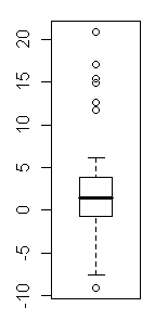
> boxplot(weight.gain.CBT)
> ### Outliers all over the place!
> weight.gain.CBT
[1] 1.7 0.7 -0.1 -0.7 -3.5 14.9 3.5 17.1 -7.6 1.6 11.7 6.1 1.1 -4.0 20.9
[16] -9.1 2.1 -1.4 1.4 -0.3 -3.7 -0.8 2.4 12.6 1.9 3.9 0.1 15.4 -0.7
> ### Excellent! Everybody changed. We now wish to test the null hypothesis
> ### that cognitive behavior therapy produces no change in median body weight
> ### when used in the treatment of anorexia.
> length(weight.gain.CBT)
[1] 29
> sum(weight.gain.CBT > 0)
[1] 18
> ### There are 29 cases in the data set, of whom 18 showed a gain. The null
> ### implies that as many women should lose weight as gain if CBT is valueless.
> ### I.e., the null implies a median weight change of zero.
> binom.test(x=18, n=29, p=1/2, alternative="greater")
Exact binomial test
data: 18 and 29
number of successes = 18, number of trials = 29, p-value = 0.1325
alternative hypothesis: true probability of success is greater than 0.5
95 percent confidence interval:
0.4512346 1.0000000
sample estimates:
probability of success
0.6206897
> detach(anorexia)
The sign test assumes a continuous variable, as it does not deal very well with
data values that happen to fall at the null hypothesized median. (They should
probably just be omitted.) It's also not an especially powerful test, as it
tosses out almost all the numerical information in the data. However, it makes
no distribution assumptions, and for that reason alone is a useful tool.
Another Alternative: The Single-Sample Wilcoxin Test
If the dependent variable is continuous and appears to be symmetrically
distributed, then more of the numerical information in the sample can be
retained by using the Wilcoxin test instead of the sign test. The syntax is
very similar to the t-test.
wilcox.test(x, y = NULL,
            alternative = c("two.sided", "less", "greater"),
            mu = 0, paired = FALSE, exact = NULL, correct = TRUE,
            conf.int = FALSE, conf.level = 0.95, ...)
The following example is based on the one on the help page for this function.
> ## Hollander & Wolfe (1973), 29f.
> ## Hamilton depression scale factor measurements in 9 patients with
> ##  mixed anxiety and depression, taken at the first (x) and second
> ##  (y) visit after initiation of a therapy (administration of a
> ##  tranquilizer).
> x = c(1.83,  0.50,  1.62,  2.48, 1.68, 1.88, 1.55, 3.06, 1.30)
> y = c(0.878, 0.647, 0.598, 2.05, 1.06, 1.29, 1.06, 3.14, 1.29)
> change = y - x                       ### expected to be negative
> change
[1] -0.952  0.147 -1.022 -0.430 -0.620 -0.590 -0.490  0.080 -0.010
> wilcox.test(change, mu=0, alternative = "less")

        Wilcoxon signed rank test

data:  change
V = 5, p-value = 0.01953
alternative hypothesis: true location is less than 0
Technically, this could also be considered a two-sample paired test, as...
wilcox.test(x, y, paired = TRUE, alternative = "greater")
...would have given the same result.
revised 2016 January 28
| Table of Contents
| Function Reference
| Function Finder
| R Project |
|