
| Table of Contents
| Function Reference
| Function Finder
| R Project |
COUNTS AND PROPORTIONS
Binomial and Poisson Data
Count data--data derived from counting things--are often treated as if they
are assumed to be binomial distributed or Poisson distributed. The binomial
model applies when the counts are derived from independent Bernoulli trials in
which the probability of a "success" is known, and the number of trials (i.e.,
the maximum possible value of the count) is also known. The classic example is
coin tossing. We toss a coin 100 times and count the number of times the coin
lands heads side up. The maximum possible count is 100, and the probability of
adding one to the count (a "success") on each trial is known to be 0.5 (assuming
the coin is fair). Trials are independent; i.e., previous outcomes do not
influence the probability of success on current or future trials. Another
requirement is that the probability of success remain constant over trials.
Poisson counts are often assumed to occur when the maximum possible count is
not known, but is assumed to be large, and the probability of adding one to the
count at each moment (trials are often ill defined) is also unknown, but is
assumed to be small. A example may help.
Suppose we are counting traffic fatalities during a given month. The maximum
possible count is quite high, we can imagine, but in advance we can't say
exactly (or even approximately) what it might be. Furthermore, the probability
of a fatal accident at any given moment in time is unknown but small. This
sounds like it might be a Poisson distributed variable. But is it?
The built in data set "Seatbelts" allows us to have a look at such a count
variable. "Seatbelts" is not a data frame, it's a time series, so extracting
the counts of fatalities will take a bit of trickery.
> Seatbelts                                 some output not shown
         DriversKilled drivers front rear   kms PetrolPrice VanKilled law
Jan 1969           107    1687   867  269  9059  0.10297181        12   0
Feb 1969            97    1508   825  265  7685  0.10236300         6   0
Mar 1969           102    1507   806  319  9963  0.10206249        12   0
Apr 1969            87    1385   814  407 10955  0.10087330         8   0
...
> deaths = as.vector(Seatbelts[,1])         # all rows of column 1 extracted as a vector
> length(deaths)
[1] 192
> mean(deaths)
[1] 122.8021
> var(deaths)
[1] 644.1386
The vector "deaths" now contains the monthly number of traffic deaths in Great
Britain during the 192 months from January 1969 through December 1984. We also
have our first indication this is not a Poisson distributed variable. In the
Poisson distribution, the mean and the variance have the same value. Let's
continue nevertheless.
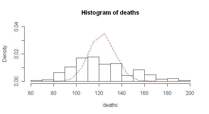
Next we'll look at a histogram of the "deaths" vector, and plotted over top
of that we will put the Poisson distribution with mean = 122.8.
> hist(deaths, breaks=15, prob=T, ylim=c(0,.04))
> lines(x<-seq(65,195,10),dpois(x,lambda=mean(deaths)),lty=2,col="red")
And I'm not gonna lie to you. That took some trial and error! The histogram
function asks for 15 break points, turns on density plotting, and sets the
y-axis to go from 0 to .04. The poisson density function was plotted using the
lines() function. The x-values were generated
by using seq() and stored into "x" on the
fly. The y-values were generated using the dpois() function. We also requested a dashed, red
line. Examination of the figure shows what we suspected. The empirical
distribution does not match the theoretical Poisson distribution.
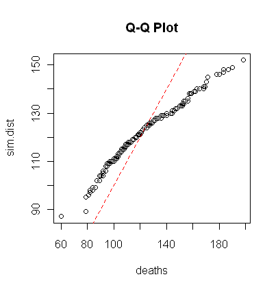
> sim.dist = rpois(192, lambda=mean(deaths))
> qqplot(deaths, sim.dist, main="Q-Q Plot")
> abline(a=0, b=1, lty=2, col="red")
Finally, you may recall (if you read that tutorial) that the qqnorm() function can be used to check a
distribution for normality. The qqplot()
function will compare any two distributions to see if they have the same shape.
If they do, the plotted points will fall along a straight line. The plot to the
right doesn't look too terribly bad until we realize these two distributions
should not only both be poisson, they should also both have the same mean (or
lambda value). Thus, the points should fall along a line with intercept 0 and
slope 1. The moral of the story: just because count data sound like they might
fit a certain distribution doesn't mean they will. R provides a number of
mechanisms for checking this.
We could have saved ourselves a lot of trouble by looking at a time series
plot to begin with. I will not reproduce it, but the command for doing so is
below. In the plot, we see the data are strongly cyclical and, therefore, that
the individual elements of the vector should not be considered independent
counts. In fact, there is a yearly cycle in the number of traffic deaths.
> plot(Seatbelts[,1]) # Not shown.
Furthermore, a scatterplot of "deaths" against its index values appears to show
that the probability of dying in a traffic accident is decreasing over the
duration of the record.
> scatter.smooth(1:192, deaths) # Not shown.
So there are lot's of problems with the poisson model here!
The Binomial Test
Suppose we set up a classic card-guessing test for ESP using a 25-card deck
of Zener cards, which consists of 5 cards each of 5 different symbols. If the
null hypothesis is correct (H0: no ESP) and the subject is just
guessing at random, then we should expect pN correct guesses from N independent
Bernoulli trials on which the probability of a success (correct guess) is
p = 0.2. Suppose our subject gets 9 correct guesses. Is this out of
line with what we should expect just by random chance?
A number of proportion tests could be applied here, but the sample size is
fairly small (just 25 guesses), so an exact binomial test is our best choice.
> binom.test(x=9, n=25, p=.2)

        Exact binomial test

data:  9 and 25
number of successes = 9, number of trials = 25, p-value = 0.07416
alternative hypothesis: true probability of success is not equal to 0.2
95 percent confidence interval:
 0.1797168 0.5747937
sample estimates:
probability of success
                  0.36
Oh, too bad! Assuming we set alpha at the traditional value of .05, we fail to
reject the null hypothesis with an obtained p-value of .074. The 95% confidence
interval tells us this subject's true rate of correct guessing is best
approximated as being between 0.18 and 0.57. This incorporates the null value of
0.2, so once again, we must regard the results as being consistent with the null
hypothesis.
We might argue at this point that we should have done a one-tailed test. (A
two-tailed test is the default.) Of course, this decision should be made in
advance, but if the subject is displaying evidence of ESP, we would expect his
success rate to be not just different from chance but greater than chance. To
take this into account in the test, we need to set the "alternative=" option.
Choices are "less" than expected, "greater" than expected, and "two.sided"
(the default).
> binom.test(x=9, n=25, p=.2, alternative="greater")

        Exact binomial test

data:  9 and 25
number of successes = 9, number of trials = 25, p-value = 0.04677
alternative hypothesis: true probability of success is greater than 0.2
95 percent confidence interval:
 0.2023778 1.0000000
sample estimates:
probability of success
                  0.36
The one-tailed test allows the null to be rejected at alpha=.05. The confidence
interval says the subject is guessing with a success rate of at least 0.202.
The confidence level can also be set by changing the "conf.level=" option to
any reasonable value less than 1. The default value is .95.
The Single-Sample Proportion Test
The subject keeps guessing because, of course, we'd like to see this above
chance performance repeated. He has now made 400 passes through the deck for a
total of 10,000 independent guesses. He has guessed correctly 2,022 times. What
should we conclude?
An exact binomial test is probably not the best choice here as the sample
size is now very large. We'll substitute a single-sample proportion test.
> prop.test(x=2022, n=10000, p=.2, alternative="greater")

        1-sample proportions test with continuity correction

data:  2022 out of 10000, null probability 0.2
X-squared = 0.2889, df = 1, p-value = 0.2955
alternative hypothesis: true p is greater than 0.2
95 percent confidence interval:
 0.1956252 1.0000000
sample estimates:
     p
0.2022
The syntax is exactly the same. Notice the proportion test calculates a
chi-squared statistic. The traditional z-test of a proportion is not implemented
in R, but the two tests are exactly equivalent. Notice also a correction for
continuity is applied. If you don't want it, set the "correct=" option to FALSE.
The default value is TRUE. (This option must be set to FALSE to make the test
mathematically equivalent to the uncorrected z-test of a proportion.)
Two-Sample Proportions Test
A random sample of 428 adults from Myrtle Beach reveals 128 smokers. A random
sample of 682 adults from San Francisco reveals 170 smokers. Is the proportion
of adult smokers in Myrtle Beach different from that in San Francisco?
> prop.test(x=c(128,170), n=c(428,682), alternative="two.sided", conf.level=.99)

        2-sample test for equality of proportions with continuity correction

data:  c(128, 170) out of c(428, 682)
X-squared = 3.0718, df = 1, p-value = 0.07966
alternative hypothesis: two.sided
99 percent confidence interval:
 -0.02330793  0.12290505
sample estimates:
   prop 1    prop 2
0.2990654 0.2492669
The two-proportions test
also does a chi-square test with continuity correction, which is mathematically
equivalent to the traditional z-test with correction. Enter "hits" or successes
into the first vector ("x"), the sample sizes into the second vector ("n"), and
set options as you like. To turn off the continuity correction, set
"correct=F". I set the alternative to two-sided, but this was unnecessary as
two-sided is the default. I also set the confidence level for the confidence
interval to 99% to illustrate this option. I made up these data, by the
way.
R incorporates a function for calculating the power of a 2-proportions test.
The syntax is illustrated here from the help page.
power.prop.test(n = NULL, p1 = NULL, p2 = NULL, sig.level = 0.05, power = NULL,
                alternative = c("two.sided", "one.sided"),
                strict = FALSE)
The value of n should be set to the sample size per group, p1 and p2 to
the group probabilities or proportions of successes, and power to the desired
power. One and only one of these options must be passed as NULL, and R will
calculate it from the others. In the example above, what sample sizes should we
have if we want a power of 90%?
> power.prop.test(p1=.299, p2=.249, sig.level=.05, power=.9,
+                 alternative="two.sided")

     Two-sample comparison of proportions power calculation

              n = 1670.065
             p1 = 0.299
             p2 = 0.249
      sig.level = 0.05
          power = 0.9
    alternative = two.sided

 NOTE: n is number in *each* group
We would need 1,670 subjects in each group.
Multiple Proportions Test
The two-proportions test generalizes directly to a multiple proportions test.
The example from the help page should suffice to illustrate.
> example(prop.test)

> ## Data from Fleiss (1981), p. 139.
> ## H0: The null hypothesis is that the four populations from which
> ##     the patients were drawn have the same true proportion of smokers.
> ## A:  The alternative is that this proportion is different in at
> ##     least one of the populations.
>
> smokers  <- c( 83, 90, 129, 70 )
> patients <- c( 86, 93, 136, 82 )
> prop.test(smokers, patients)

        4-sample test for equality of proportions without continuity
        correction

data:  smokers out of patients
X-squared = 12.6004, df = 3, p-value = 0.005585
alternative hypothesis: two.sided
sample estimates:
   prop 1    prop 2    prop 3    prop 4
0.9651163 0.9677419 0.9485294 0.8536585
If you run this example, you will notice that I have deleted some of the output
from the simpler proportion tests.
revised 2016 January 27
| Table of Contents
| Function Reference
| Function Finder
| R Project |
|