R Tutorials by William B. King, Ph.D.
| Table of Contents | Function Reference | Function Finder | R Project |

MULTIPLE COMPARISONS, CONTRASTS, AND POST HOC TESTS


Don't those three things kind of overlap with one another? I mean, aren't post hoc tests also multiple comparisons? Sure they are. I just wanted to make sure I was catching everyone who is interested in one or another of these topics, regardless of what they decide to call it.

When it comes to multiple comparisons, R is both rich and poor. The base packages are quite limited (but still offer some powerful choices). However, there are optional packages that can be downloaded from CRAN that will do just about anything any sane person might want. One that I can recommend is a package called "multcomp". In this tutorial, I'm going to stick to what's available in the base packages.

Furthermore, in this tutorial I'm going to stick to looking at one main effect, as might result from a one-way ANOVA, and main effects from between groups designs at that. I think it's necessary to cover this material first, before more complex situations can be tackled. We will tackle those in the relevant tutorials on factorial ANOVA and repeated measures designs.

A note: For some of the things in this tutorial to work, it is necessary to have your contrasts for unordered factors set to "treatment contrasts", which is the R default. You can check that as follows:

> options("contrasts")
$contrasts
        unordered           ordered 
"contr.treatment"      "contr.poly" 

> ### if you don't see "contr.treatment" under unordered, do this
> options(contrasts = c("contr.treatment","contr.poly"))


Post Hoc Tests

Post hoc tests are done after an omnibus ANOVA has been completed, when there has been a significant effect, and now it is desired to see exactly which groups are significantly different. Statisticians thrive on post hoc tests. There are more of these things than you can shake a stick at! Or would even care to shake a stick at!! I'm going to discuss four: the Tukey HSD test, the Fisher LSD test (with a note on Dunnett's test), the Bonferroni test, and the Holm-Bonferroni test.

Tukey HSD test

The Tukey Honestly Significant Difference test was illustrated in the Oneway Between Subjects ANOVA tutorial. I'll repeat that example here. Briefly, we are testing six insect sprays, A through F, and after we spray garden plots with them, we are counting how many bugs are left.

> aov.out = aov(count ~ spray, data=InsectSprays)
> TukeyHSD(aov.out)                    # just run TukeyHSD() on the model object
  Tukey multiple comparisons of means
    95% family-wise confidence level

Fit: aov(formula = count ~ spray, data = InsectSprays)

$spray
           diff        lwr       upr     p adj
B-A   0.8333333  -3.866075  5.532742 0.9951810
C-A -12.4166667 -17.116075 -7.717258 0.0000000
D-A  -9.5833333 -14.282742 -4.883925 0.0000014
E-A -11.0000000 -15.699409 -6.300591 0.0000000
F-A   2.1666667  -2.532742  6.866075 0.7542147
C-B -13.2500000 -17.949409 -8.550591 0.0000000
D-B -10.4166667 -15.116075 -5.717258 0.0000002
E-B -11.8333333 -16.532742 -7.133925 0.0000000
F-B   1.3333333  -3.366075  6.032742 0.9603075
D-C   2.8333333  -1.866075  7.532742 0.4920707
E-C   1.4166667  -3.282742  6.116075 0.9488669
F-C  14.5833333   9.883925 19.282742 0.0000000
E-D  -1.4166667  -6.116075  3.282742 0.9488669
F-D  11.7500000   7.050591 16.449409 0.0000000
F-E  13.1666667   8.467258 17.866075 0.0000000
The test is of pairwise comparisons, B with A, C with A, etc. For each comparison, the test reports the diff(erence) between the group means, a 95% confidence interval thereupon, and a p-value that has been adjusted by the Tukey method for the number of comparisons being made. The Tukey test is fairly conservative in controlling familywise error rate, and for that reason it does not have to be protected. (I.e., you can do the Tukey HSD test even without a signicant effect in the omnibus ANOVA, although there would rarely be any point. There might be more of a point in doing the Tukey HSD test instead of the omnibus ANOVA.)

What you don't get in this output is the actual HSD value. You don't really need it, unless your homework requires that you calculate it! Which would not be difficult. It's half the width of any of those CIs. (Notice they are all the same width.)

> (5.532742-(-3.866075))/2             # HSD value from the B-A result
[1] 4.699408
If you want a visual representation of the tests, that is easily enough obtained as well.
> plot(TukeyHSD(aov.out), las=1)       # las=1 just turns the axis labels
Tukey HSD plot
Further note: If you have more than one effect, you can specify which effect you want to be tested. Say you have an AxB factorial design, and you want tests on the A effect. You'd do it by setting an option: which="A".

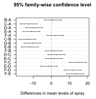
Also, the Tukey HSD test was originally intended for balanced designs only. The extention to unbalanced designs was developed by Kramer and has been incorporated into the R function. In the case of unbalanced designs, the proper name of the test is the Tukey-Kramer procedure.

Fisher LSD test

When I start talking about this test, my students immediately perk up, until I tell them that LSD stands for Least Significant Difference. The LSD test uses unadjusted p-values, and therefore it makes no attempt to control familywise error rate. If you use it as a protected test (i.e., only after seeing a significant effect in the omnibus ANOVA), it's good for about three or four comparisons without inflating the error rate. Beyond that, the inflation grows rapidly with increasing numbers of comparisons, if you're concerned about such a thing. It is among the most powerful of post hoc tests, however, and hey! Type II errors are errors too!

Fisher LSD p-values for all possible pairwise comparisons can be obtained this way.

> with(InsectSprays, pairwise.t.test(x=count, g=spray, p.adjust="none"))       # x=DV, g=IV

	Pairwise comparisons using t tests with pooled SD 

data:  count and spray 

  A       B       C       D       E      
B 0.604   -       -       -       -      
C 7.3e-11 8.5e-12 -       -       -      
D 9.8e-08 1.2e-08 0.081   -       -      
E 2.8e-09 3.3e-10 0.379   0.379   -      
F 0.181   0.408   2.8e-13 4.0e-10 1.1e-11

P value adjustment method: none
That's all you get though is just the p-values. You can get SOME of the tests this way.
> summary.lm(aov.out)$coef             # summary.lm(aov.out) is sufficient, but there is more output
               Estimate Std. Error    t value     Pr(>|t|)
(Intercept)  14.5000000   1.132156 12.8074279 1.470512e-19
sprayB        0.8333333   1.601110  0.5204724 6.044761e-01
sprayC      -12.4166667   1.601110 -7.7550382 7.266893e-11
sprayD       -9.5833333   1.601110 -5.9854322 9.816910e-08
sprayE      -11.0000000   1.601110 -6.8702352 2.753922e-09
sprayF        2.1666667   1.601110  1.3532281 1.805998e-01
Those are tests against the "missing level" of the factor. I.e., spray A doesn't appear in this table, so these tests are A-B, A-C, A-D, A-E, and A-F. (This assumes you have your contrasts set to "treatment," which is the R default. Check with options("contrasts") and look at what it says for unordered factors.) Compare the p-values to those above in the first column of the pairwise t-tests.

How would we get the other comparisons? One way would be to calculate them by hand, which is not difficult using the information above. The LSD test is done as a t-test, with t equal to the difference in the means of the two groups that are being compared, divided by the standard error of that difference. The standard error is defined this way:

s * sqrt(1/n1 + 1/n2)

Where n1 and n2 are the two group sizes, both 12 in this case, and s is the pooled standard deviation of the treatment groups, which can be obtained as follows.
> aov.out
Call:
   aov(formula = count ~ spray, data = InsectSprays)

Terms:
                   spray Residuals
Sum of Squares  2668.833  1015.167
Deg. of Freedom        5        66

Residual standard error: 3.921902      # this is sqrt(1015.167/66) or sqrt of the MSE term
Estimated effects may be unbalanced

> 3.921902/sqrt(6)                     # calculation of se; /sqrt(6) being from sqrt(1/12 + 1/12)
[1] 1.60111
Notice the result matches that in the summary.lm table above. With a balanced design, n1 and n2 are the same for all comparisons, and s is the same for all comparisons, so the standard error will always be the same. Furthermore, the difference in means between any two groups can be obtained from the "Estimates" in the above table. So let's say we wanted the comparison between spray D and spray E. We would do it this way.
> (-9.5833333 - (-11.0)) / 1.601110    # t
[1] 0.8848029
> pt(0.8848029, df=66, lower=F) * 2    # two-tailed p-value (drop any sign on t)
[1] 0.3794751
Compare this to the p-value in the pairwise t-test table.

When the design is unbalanced, the same standard error will not be used for all tests in the summary.lm output. Neither will it be in the pairwise t-tests. This is because n1 and n2 may vary between comparisons. Let's unbalance the InsectSprays data, and see what effect that has. We'll drop 5 cases selected at random.

> InSpr = InsectSprays[-sample(1:72,5),]
> summary(InSpr)                       # your result will be different
     count        spray 
 Min.   : 0.000   A:12  
 1st Qu.: 3.000   B:11  
 Median : 7.000   C:12  
 Mean   : 9.582   D:12  
 3rd Qu.:14.500   E: 9  
 Max.   :26.000   F:11
> with(InSpr, tapply(count,spray,mean))
        A         B         C         D         E         F 
14.500000 14.818182  2.083333  4.916667  3.555556 17.181818 
> aov.unb = aov(count ~ spray, data=InSpr)
> summary.lm(aov.unb)$coef
               Estimate Std. Error   t value     Pr(>|t|)
(Intercept)  14.5000000   1.128571 12.848106 5.262536e-19
sprayB        0.3181818   1.631911  0.194975 8.460605e-01
sprayC      -12.4166667   1.596040 -7.779669 1.053451e-10
sprayD       -9.5833333   1.596040 -6.004443 1.148894e-07
sprayE      -10.9444444   1.723921 -6.348578 3.010487e-08
sprayF        2.6818182   1.631911  1.643361 1.054535e-01
> with(InSpr, pairwise.t.test(x=count, g=spray, p.adjust="none"))

	Pairwise comparisons using t tests with pooled SD 

data:  count and spray 

  A       B       C       D       E      
B 0.846   -       -       -       -      
C 1.1e-10 9.6e-11 -       -       -      
D 1.1e-07 9.0e-08 0.081   -       -      
E 3.0e-08 2.4e-08 0.396   0.433   -      
F 0.105   0.161   3.2e-13 3.0e-10 1.2e-10

P value adjustment method: none
So with an unbalanced design, a little more calculation would be involved to get non-A comparison t-values.

Is there a way to get those other, non-A, comparisons? Other than doing them by hand, that is? Because hey! What do I own a computer for? The pairwise.t.test() function gives the p-values for them, but if you insist on having all the gory details, that's another matter.

They can be had though if you're willing to do a little work. Let's say we want all the B-comparisons. The reasons we got A-comparisons above is because A is the first level of the spray factor.

> levels(InsectSprays$spray)
[1] "A" "B" "C" "D" "E" "F"
If we could make B the first level, then we could get the B-comparisons. Easy peasy!
> Bspray = relevel(InsectSprays$spray, ref="B")       # "reference group" is now B
> levels(Bspray)
[1] "B" "A" "C" "D" "E" "F"
> summary.lm(aov(InsectSprays$count ~ Bspray))$coef   # the ANOVA must be recalculated
               Estimate Std. Error    t value     Pr(>|t|)
(Intercept)  15.3333333   1.132156 13.5434869 1.001994e-20
BsprayA      -0.8333333   1.601110 -0.5204724 6.044761e-01
BsprayC     -13.2500000   1.601110 -8.2755106 8.509776e-12
BsprayD     -10.4166667   1.601110 -6.5059045 1.212803e-08
BsprayE     -11.8333333   1.601110 -7.3907075 3.257986e-10
BsprayF       1.3333333   1.601110  0.8327558 4.079858e-01
And so on.

The LSD (least significant difference) can be calculated this way.

> alpha = .05
> s = 3.921902                         # from the aov output, this is sqrt of MSE
> df = 66                              # also from the aov output, df error
> tcrit = qt(p=1-alpha/2, df=df)
> LSD = tcrit * s * sqrt(1/12+1/12)    # reciprocals of the group sizes, each group is n=12
> LSD
[1] 3.196719
Since all the group sizes are 12 (in the balanced data), this would be the LSD for all comparisons. If the data are unbalanced, then there would be several LSDs, depending upon which groups were being compared.

What about confidence intervals? If you have LSD, a confidence interval is just one more step. Let's do the 95%-CI for the D-E mean difference.

> summary.lm(aov.out)$coef             # because I don't like to scroll
               Estimate Std. Error    t value     Pr(>|t|)
(Intercept)  14.5000000   1.132156 12.8074279 1.470512e-19
sprayB        0.8333333   1.601110  0.5204724 6.044761e-01
sprayC      -12.4166667   1.601110 -7.7550382 7.266893e-11
sprayD       -9.5833333   1.601110 -5.9854322 9.816910e-08
sprayE      -11.0000000   1.601110 -6.8702352 2.753922e-09
sprayF        2.1666667   1.601110  1.3532281 1.805998e-01
> (-9.5833333 - (-11.0)) - LSD         # lower bound
[1] -1.780052
> (-9.5833333 - (-11.0)) + LSD         # upper bound
[1] 4.613386

A note on Dunnett's test

Notice above when you did summary.lm(aov.out), you got comparisons of group A with groups B, C, D, E, and F in turn. If group A is your control group, then these are Dunnett-like tests of all treatment groups with the control. The tests themselves are wrong, however, because Dunnett's adjustment to the p-value was not done.

So far as I'm aware, there is no way to do it in the R base packages. There are optional packages that can be downloaded from CRAN that will do it, one of which is "multcomp". There are also tables of Dunnett's critical values online, for example, here.

Bonferroni test

The Bonferroni test is done exactly like the Fisher LSD test, but once the p-values are obtained, they are multiplied by the number of comparisons being made. In the case of InsectSprays, that would be 15 comparisons. The p-values for all the comparisons can be obtained like this.

> with(InsectSprays, pairwise.t.test(x=count, g=spray, p.adjust="bonferroni"))

	Pairwise comparisons using t tests with pooled SD 

data:  count and spray 

  A       B       C       D       E      
B 1       -       -       -       -      
C 1.1e-09 1.3e-10 -       -       -      
D 1.5e-06 1.8e-07 1       -       -      
E 4.1e-08 4.9e-09 1       1       -      
F 1       1       4.2e-12 6.1e-09 1.6e-10

P value adjustment method: bonferroni
Note: Any p-values that come out greater than 1 due to the multiplication are set at 1. You can't have a p-value greater than one (unless you're one of my students). The Bonferroni test is very conservative and does not require protection.

Holm-Bonferroni test

The Holm-Bonferroni test is a very clever modification of the Bonferroni correction. For details you'll have to consult a textbook (or Wikipedia), but here is how you get the p-values.

> with(InsectSprays, pairwise.t.test(x=count, g=spray, p.adjust="holm"))

	Pairwise comparisons using t tests with pooled SD 

data:  count and spray 

  A       B       C       D       E      
B 1.00    -       -       -       -      
C 8.7e-10 1.2e-10 -       -       -      
D 6.9e-07 9.7e-08 0.49    -       -      
E 2.5e-08 3.6e-09 1.00    1.00    -      
F 0.90    1.00    4.2e-12 4.0e-09 1.4e-10

P value adjustment method: holm
Holm is actually the default for the p-adjustment method in this function, so it would not need to be specified explicitly. The Holm test is much less conservative than the Bonferroni test but not so much that it requires protection. It does not.


Orthogonal Contrasts

Clean up your workspace and search path. We're moving on to a new problem.

We will look at a data set that records the dry-weight production of biomass by plants as the result of three different treatments: a control, and two experimental treatments.

> data(PlantGrowth)
> summary(PlantGrowth)
     weight       group   
 Min.   :3.590   ctrl:10  
 1st Qu.:4.550   trt1:10  
 Median :5.155   trt2:10  
 Mean   :5.073            
 3rd Qu.:5.530            
 Max.   :6.310            
> with(PlantGrowth, tapply(weight, group, mean))
 ctrl  trt1  trt2 
5.032 4.661 5.526 
> with(PlantGrowth, tapply(weight, group, var))
     ctrl      trt1      trt2 
0.3399956 0.6299211 0.1958711 
> with(PlantGrowth, bartlett.test(weight ~ group))

        Bartlett test of homogeneity of variances

data:  weight by group 
Bartlett's K-squared = 2.8786, df = 2, p-value = 0.2371
The design is balanced, a necessary prerequisite for orthogonal contrasts, and although there are substantial differences in the group variances, Bartlett's test does not reveal a significant deviation from homogeneity of variance.

Okay, stop! Don't go rushing headlong into the ANOVA without stopping and thinking first. What kind of hypotheses might we be interested in here? Well, any differences among the means. That's the traditional alternative for the omnibus ANOVA, but it's really kind of like beating the problem with a club!

If we think about it, we might come up with hypotheses like these: (i) the treated groups will be different from the control group, and (ii) the two treated groups will be different from each other. (NOTE: Given that I don't know what the treatments are, I don't know if these are sensible hypotheses, but they COULD be. Use your imagination.)

These are hypotheses which, like all hypotheses, we would want to express in advance. And now we want to come up with a method of data analysis that would allow us to test them. Enter what are called planned comparisons. The name makes perfect sense, since we're planning these comparisons in advance. We'll use contrasts to do the analysis.

Contrasts do not have to be "orthogonal." Think of orthogonal as meaning something like "independent" or "unconfounded." I'll discuss nonorthogonal contrasts below. Right now, let's keep our contrasts orthogonal.

There are several requirements for doing so. One has already been mentioned: a balanced design, which means orthogonal contrasts are done most often on experimental data (as opposed to quasi-experiments). Another one is that we can come up with a set of k-1 sensible orthogonal contrasts, where k is the number of levels of the IV we are testing. In this case, our IV has three levels, so we can have two contrasts, each corresponding to a sensible hypothesis. I think we have that. It now remains to code the contrasts.

Each contrast is going to be coded with a contrast vector. Within the vector, each level of the IV is going to be given a code. Some of the codes will be positive, some will be negative. All of the positive codes in the vector should be the same, and they should add to +1. All of the negative codes in the vector should be the same, and they should add to -1. Thus, the codes in the vector should, overall, add to 0.

The positively coded groups will be combined into one big "megagroup." The negatively coded groups will be combined into another big "megagroup." Then these two megagroups will be tested against each other, using what essentially amounts to a t-test. This is called a complex contrast, by the way, when you have groups combined into megagroups. A contrast can also just test one group against another, which is called a simple contrast. Fisher LSD tests are simple contrasts.

Our first hypothesis suggests we want to lump the treatment groups into a megagroup, and test that megagroup against the control group. The contrast vector would be:

< +1, -1/2, -1/2 >

These codes have to be in the SAME ORDER that R sees the levels of the variable, so we better check that.
> levels(PlantGrowth$group)
[1] "ctrl" "trt1" "trt2"
Good! Our contrast will test "ctrl" (+1) against the megagroup "trt1+trt2" (each coded -1/2). "That's not going to give us anything," you're saying. "I've seen the means, and that's just not going to pan out!" Stop looking at the means! These are PLANNED in advance comparisons. You haven't got any means yet!

For our second hypothesis, we want to compare "trt1" to "trt2". The secret here is to code any level not included in the contrast as 0. So the vector is:

< 0, +1, -1 >

That will compare the second level of the IV to the third level, a simple contrast and, FYI, equivalent to a Fisher LSD test. By the way, it's completely arbitrary which levels are coded positive and which negative, but I'll give you a hint below as to what is a convenient way to choose.
> vec1 = c(1,-1/2,-1/2)
> vec2 = c(0,1,-1)
> ### now cbind the contrast vectors into the columns of matrix
> cons = cbind(vec1, vec2)
> cons
     vec1 vec2
[1,]  1.0    0
[2,] -0.5    1
[3,] -0.5   -1
> ### it's helpful (but not really necessary) to name the rows of the matrix
> rownames(cons) = c("ctrl", "trt1", "trt2")
> cons
     vec1 vec2
ctrl  1.0    0
trt1 -0.5    1
trt2 -0.5   -1
> ### to be orthogonal, all pairs of contrast vectors must have a dot product of 0
> ### here's a convenient way to test that for a contrast matrix of any size
> t(cons) %*% cons
     vec1 vec2
vec1  1.5    0
vec2  0.0    2
> ### if this matrix multiplication results in a matrix that is nonzero ONLY on
> ### the main diagonal, then the contrasts are orthogonal
And we are coded! Now we assign that contrast matrix to the IV and run the ANOVA. We're not really interested in the ANOVA itself, but this is how we're going to get the contrasts.
> contrasts(PlantGrowth$group) = cons
> aov.out = aov(weight ~ group, data=PlantGrowth)
Now here's the tricky part. I'll do it, and then I'll explained what happened.
> summary(aov.out, 
+         split=list(
+            group=list("ctrl v trts"=1, "trt1 v trt2"=2)
+          ))
                     Df Sum Sq Mean Sq F value  Pr(>F)   
group                 2  3.766   1.883   4.846 0.01591 * 
  group: ctrl v trts  1  0.025   0.025   0.065 0.80086   
  group: trt1 v trt2  1  3.741   3.741   9.627 0.00446 **
Residuals            27 10.492   0.389                   
---
Signif. codes:  0 '***' 0.001 '**' 0.01 '*' 0.05 '.' 0.1 ' ' 1
I get that wrong EVERY time! I always have to look at an example. We used the usual extractor function, summary(aov.out), but this time we used it with an option called split=. The technical statistical jargon for what split does is "partition." Our contrasts partitioned the treatment sum of squares. Because we had a full set of orthogonal contrasts, the partitioning was spot on. I.e., the contrast SSs add up to the treatment SS. What's up with that syntax?!

For once, it's actually quite sensible. Inside split we have a list that lists ALL of the factors we're doing contrasts on. Here we only have one, so our list exhausted itself at "group." Inside each of those factors we have another list. In that list, we give our contrasts sensible names, and we set those names equal to one of the columns in the contrast matrix (by number of the column). And that's pretty much it.

"I thought you said they were like t-tests. That don't look like no t-test to me!"

> summary.lm(aov.out)$coef
            Estimate Std. Error    t value     Pr(>|t|)
(Intercept)   5.0730  0.1138121 44.5734621 8.020008e-27
groupvec1    -0.0410  0.1609546 -0.2547302 8.008617e-01
groupvec2    -0.4325  0.1393908 -3.1027872 4.459236e-03
The "estimates" are meaningless. They do have something to do with the differences in the means, but it's best not to go there! The t-values are the square roots of the corresponding F-values in the previous table (ignoring signs), and the p-values are the same. The degrees of freedom for the t-tests is just the error df from the onmibus ANOVA (27 in this case). The intercept is the overall (grand) mean, and it is significantly different from 0, but who cares?

Here is another brief example. The data are based on an experiment by Eysenck (1974) on incidental learning, which is learning that takes place when one is not really attempting to learn but just through exposure to the material. Subjects were given a list of 30 words and one of five different instructions: count the letters in each word, think of a word that rhymes with each word, think of an adjective that could be used to modify the word in a sentence, form a mental image of the object described by the word, or a control condition in which the subjects were told to memorize the list. These are not the original data but were created to match the cell means and SDs. The data were taken from Howell's textbook (7th ed., 2010, Table 11.1, p. 319).

The logic of the following contrasts is that only the control group was told they'd be asked to recall the words, and that count and rhyme instructions represent a shallow level of mental processing, while adjective and image instructions represent deep mental processing. (Note: In the full experiment, there were two age groups. These data are for the older subjects.)

> scores = scan()
1:  9  8  6  8 10  4  6  5  7  7       # count instructions
11: 7  9  6  6  6 11  6  3  8  7       # rhyme instructions
21: 11 13 8  6 14 11 13 13 10 11       # adjective instructions
31: 12 11 16 11 9 23 12 10 19 11       # image instructions
41: 10 19 14 5 10 11 14 15 11 11       # control instructions
51: 
Read 50 items
> ### btw, trying to put comments into a scan operation like that will fail!
> groups = gl(n=5,           # generate levels, n=no. of levels
+             k=10,          # k=replications per group
+             labels=c("count","rhyme","adjec","image","contr"))
> levels(groups)
[1] "count" "rhyme" "adjec" "image" "contr"
> c1=c(-1/4,  -1/4,   -1/4,   -1/4,   +1)   # control vs. treatments
> c2=c(-1/2,  -1/2,   +1/2,   +1/2,    0)   # shallow vs. deep processing
> c3=c(   0,     0,     -1,     +1,    0)   # are the deep processing conditions different
> c4=c(  -1,    +1,      0,      0,    0)   # are the shallow processing conditions different
> cons  = cbind(c1, c2, c3, c4)
> rownames(cons) = levels(groups)
> cons
         c1   c2 c3 c4
count -0.25 -0.5  0 -1
rhyme -0.25 -0.5  0  1
adjec -0.25  0.5 -1  0
image -0.25  0.5  1  0
contr  1.00  0.0  0  0
> contrasts(groups) = cons
> aov.out = aov(scores ~ groups)       # do this AFTER contrasts are assigned
> summary(aov.out, split=list(
+      groups=list("cont-treat"=1, "shallow-deep"=2,
+                  "deep-deep"=3, "shallow-shallow"=4)
+ ))
                          Df Sum Sq Mean Sq F value   Pr(>F)    
groups                     4  351.5   87.88   9.085 1.82e-05 ***
  groups: cont-treat       1   47.0   47.05   4.863   0.0326 *  
  groups: shallow-deep     1  275.6  275.63  28.493 2.96e-06 ***
  groups: deep-deep        1   28.8   28.80   2.977   0.0913 .  
  groups: shallow-shallow  1    0.0    0.05   0.005   0.9430    
Residuals                 45  435.3    9.67                     
---
Signif. codes:  0 '***' 0.001 '**' 0.01 '*' 0.05 '.' 0.1 ' ' 1
>  summary.lm(aov.out)       # forgot $coef so we'll get full output

Call:
aov(formula = scores ~ groups)

Residuals:
   Min     1Q Median     3Q    Max 
 -7.00  -1.85  -0.45   2.00   9.60 

Coefficients:
            Estimate Std. Error t value Pr(>|t|)    
(Intercept)  10.0600     0.4399  22.872  < 2e-16 ***
groupsc1      1.9400     0.8797   2.205   0.0326 *  
groupsc2      5.2500     0.9835   5.338 2.96e-06 ***
groupsc3      1.2000     0.6955   1.725   0.0913 .  
groupsc4     -0.0500     0.6955  -0.072   0.9430    
---
Signif. codes:  0 '***' 0.001 '**' 0.01 '*' 0.05 '.' 0.1 ' ' 1 

Residual standard error: 3.11 on 45 degrees of freedom
Multiple R-squared: 0.4468,	Adjusted R-squared: 0.3976 
F-statistic: 9.085 on 4 and 45 DF,  p-value: 1.815e-05
One new function here, gl(), which means generate levels for a balanced design. The syntax is kind of goofy in that n stands for the number of levels of the IV, while k stands for the number of replicates (subjects per group). Much more common statistical notation would have that the other way around, so don't get confused.

  • Eysenck, Michael W. Age differences in incidental learning. Developmental Psychology, Vol 10(6), Nov 1974, 936-941.
  • Howell, David C. Statistical Methods for Psychology (7th ed.). Belmont, CA: Cengage Wadsworth, 2010.

Nonorthogonal Contrasts

Those are not the contrasts I would have selected for the Eysenck study, and luckily for me, the statistics police will not come and put me in statistics prison if my contrasts are not orthogonal. (I'll probably get off with a warning.)

There is no rule that says contrasts have to be orthogonal, even when the design is balanced. Here are the contrasts I would test. (Note: Contrasts are very personal things, kind of like underwear. People have different tastes. As long as those tastes correspond to sensible hypotheses, the rule is live and let live!)

> levels(groups)
[1] "count" "rhyme" "adjec" "image" "contr"
> c1=c(-1/2,  -1/2,  +1/2,   +1/2,     0)        # test shallow against deep processing
> c2=c(-1/2,  -1/2,     0,      0,     1)        # test shallow processing against control
> c3=c( 0,      0,   -1/2,   -1/2,     1)        # test deep processing against control
> cons = cbind(c1, c2, c3)
> rownames(cons) = levels(groups)
> cons
        c1   c2   c3
count -0.5 -0.5  0.0
rhyme -0.5 -0.5  0.0
adjec  0.5  0.0 -0.5
image  0.5  0.0 -0.5
contr  0.0  1.0  1.0
> t(cons) %*% cons                               # not orthogonal
     c1  c2   c3
c1  1.0 0.5 -0.5
c2  0.5 1.5  1.0
c3 -0.5 1.0  1.5
> contrasts(groups) = cons
Error in `contrasts<-`(`*tmp*`, value = c(-0.5, -0.5, 0.5, 0.5, 0, -0.5,  : 
  singular contrast matrix
Okay, I didn't get away with a warning. I got an error. So the bus stops here! (Or doesn't stop here, depending upon how you think about it!)

Yeah, I know, it annoys me, too. So I've written a function to do it (see Writing Your Own Functions and Scripts if you don't know what I'm talking about). Open a script window (File > New Script in Windows or File > New Document on a Mac), and copy and paste these lines into it.

### begin copying here
SScontrasts = function (means, contr.matrix, n, mse, dfe) 
{
    diffs = (as.vector(means) %*% contr.matrix)
    tmp1 = diffs^2/apply(contr.matrix^2/as.vector(n), 2, sum)
    tmp2 = tmp1/mse
    tmp3 = 1 - pf(tmp2, 1, dfe)
    output = rbind(tmp1, tmp2, tmp3, diffs)
    rownames(output) = c("SS", "F", "p-value", "diffs")
    output
}
### end copying here and paste
Then save the script as "SScontrasts.R" to whatever your usual working directory is (Rspace). Then, any time you want it, you just read it in like this.
> source("SScontrasts.R")              # this will put it in your workspace
You use it like this.
> means = tapply(scores,groups,mean)   # put the group means in a vector
> means
count rhyme adjec image contr 
  7.0   6.9  11.0  13.4  12.0 
> aov.out                              # you'll need some of this information, too
Call:
   aov(formula = scores ~ groups)

Terms:
                groups Residuals
Sum of Squares  351.52    435.30
Deg. of Freedom      4        45

Residual standard error: 3.110198
Estimated effects may be unbalanced

> args(SScontrasts)                    # check to see what you need to feed the function
function (means, contr.matrix, n, mse, dfe)
>   ### means is the vector of means
>   ### contr.matrix is the contrast matrix you've prepared (cons)
>   ### n is a vector of group sizes; if the design is balanced, a single number will do
>   ### mse is the mean square error term from the ANOVA table
>   ### dfe is the error degrees of freedom from the ANOVA table
>
> SScontrasts(means, cons, n=10, mse=435.3/45, dfe=45)
                  c1           c2         c3
SS      2.756250e+02 1.700167e+02  0.2666667
F       2.849328e+01 1.757581e+01  0.0275672
p-value 2.963530e-06 1.275381e-04  0.8688742
diffs   5.250000e+00 5.050000e+00 -0.2000000
The function reports a matrix of results. For each contrast (in columns) you'll get a sum of squares (these are not orthogonal contrasts, so don't expect the SS treatment to be correctly partitioned), an F value for the test (which is on 1 and dfe degrees of freedom), a p-value, and the difference in the means of the two (mega)groups being contrasted.

If you'd rather report your results as t-tests, then t = sqrt(F) on dfe degrees of freedom, with a p-value as reported in the above table. These are two-tailed p-values when it comes to the t-test. For one-tailed, divide them in half, PROVIDED the effect went in the predicted direction. If you code the group(s) that you expect to have the larger mean with positive-valued contrast codes, then "diffs" will be positive if the effect went in the direction you expected.


A Final Note

Do planned contrasts require a p-adjustment for the number of comparisons? Oh no! You're not dragging me into that argument! Just try to hold it down to a reasonable number.


created 2016 February 4
| Table of Contents | Function Reference | Function Finder | R Project |