
| Table of Contents
| Function Reference
| Function Finder
| R Project |
MORE DESCRIPTIVE STATISTICS
Categorical Data: Crosstabulations
Categorical data are summarized by counting up frequencies and
by calculating proportions and percentages.
Categorical data are commonly encountered in three forms: a frequency table
or crosstabulation, a flat table, or a case-by-case data frame. Let's begin
with the first of these.
In the default download of R, there is a data set called UCBAdmissions,
which gives admissions data for UC Berkeley's top six grad programs in 1974.
You might want to enlarge your R Console window a bit so you can see all the
data at once.
> setwd(Rspace)                   # Okay. Everybody forgets once in awhile. Give me a break!
Error in setwd(Rspace) : object 'Rspace' not found
> setwd("Rspace")                 # if you've created this directory
> UCBAdmissions
, , Dept = A

          Gender
Admit      Male Female
  Admitted  512     89
  Rejected  313     19

, , Dept = B

          Gender
Admit      Male Female
  Admitted  353     17
  Rejected  207      8

, , Dept = C

          Gender
Admit      Male Female
  Admitted  120    202
  Rejected  205    391

, , Dept = D

          Gender
Admit      Male Female
  Admitted  138    131
  Rejected  279    244

, , Dept = E

          Gender
Admit      Male Female
  Admitted   53     94
  Rejected  138    299

, , Dept = F

          Gender
Admit      Male Female
  Admitted   22     24
  Rejected  351    317
This is a three-dimensional table, specifically a 2x2x6 contingency table. In
R, the dimensions are recognized in this order: rows (the "Admit" variable in
this table), columns (the "Gender" variable in this table), and layers (the
"Dept" variable in this table). The numbers in the table are frequencies, for
example, how many male applicants admitted to department A (512). We don't have
information on individual subjects, but if we did, the first one of them would
be someone who was admitted, would be male, and would have applied to dept. A,
and that would be it. Thus, you can see that the frequency table, or crosstabs,
contains complete information on our subjects.
How would we create this table ourselves? Well, we would start with all of
those numbers in a vector. The tricky part is getting them in the correct order,
and to do that we need to know in what order R is going to stick them into the
table. R will pick a layer of the table, beginning with the first one (A), and
fill down the columns, then move to the next layer and fill down the columns,
and so on. Thus, when the admissions office at Berkeley sends us these numbers,
we want to create the following vector from them. (Use
scan() to enter the vector if you prefer. I'm going to use c() because it will keep things clearer, hopefully.)
> OF = c(512, 313,  89,  19,   # Dept A, males adm, males rej, females adm, females rej
+        353, 207,  17,   8,   # Dept B
+        120, 205, 202, 391,   # Dept C
+        138, 279, 131, 244,   # Dept D
+         53, 138,  94, 299,   # Dept E
+         22, 351,  24, 317)   # Dept F
Yes, you can bet I spaced it just like that, and I included the comments. When I
come back and look at this later, I want to know exactly what I did! Another
confession: If I get one of those numbers wrong, I don't want to have to retype
the whole gosh darned thing! So I typed it into a script window (no command
prompts typed there), and then copied and pasted it into R, a good way to deal
with long commands, and also the way I'm going to deal with the next one! (To
get a script window, go to File > New Script in Windows, or File > New Document
on a Mac, or open a text editor in Linux.) So my
entire script looks like this, which you can copy and paste if your fingers are
broken and you can't type today:
OF = c(512, 313,  89,  19,   # Dept A, males adm, males rej, females adm, females rej
       353, 207,  17,   8,   # Dept B
       120, 205, 202, 391,   # Dept C
       138, 279, 131, 244,   # Dept D
        53, 138,  94, 299,   # Dept E
        22, 351,  24, 317)   # Dept F
UCB = array(data=OF, dim=c(2,2,6), dimnames=list(
       Admit=c("admitted","rejected"),
       Gender=c("male","female"),
       Dept=c("A","B","C","D","E","F")
       ))
I could also have used array() and dimnames() separately, as follows.
UCB = array(data=OF, dim=c(2,2,6))
dimnames(UCB) = list(
       Admit=c("admitted","rejected"),
       Gender=c("male","female"),
       Dept=c("A","B","C","D","E","F"))
Print out (to the Console) the table this creates in your workspace and
confirm it is the same as the one above.
Is this table arranged the way you really want it? I.e., do you really want
Admit in the rows, Gender in the columns, and Dept in the layers? Maybe you do,
but then again, maybe you don't. I think the most interesting problem here is
to compare admission by gender.
If that's what we're interested in, then why don't we just collapse the table
across (or over) departments. That would be easy enough to do, but we need to
remember that, in R, each dimension of the table has a number, and that rows
are 1, columns are 2, and layers are 3. Then we can use the margin.table() function to collapse.
> margin.table(UCB, margin=c(1,2))     # omit the "margin" that you want to collapse over
          Gender
Admit      male female
  admitted 1198    557
  rejected 1493   1278
> margin.table(UCB, margin=c(2,1))     # put Gender in the rows and Admit in the columns
        Admit
Gender   admitted rejected
  male       1198     1493
  female      557     1278
> margin.table(UCB, margin=c(2,1)) -> Admit.by.Gender      # store that second one
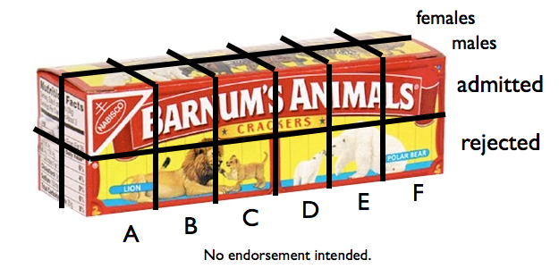
The name of the command is more sensible than it may seem at first blush. If
you can imagine what the 3D table looks like in 3D, it would resemble a box of
crackers. The box is divided into 2x2x6=24 little cells, and each cell has a
frequency in it. At the end of the box there is a margin (also above and in
front). We're going to fill that margin with sums by adding frequencies across
the length of the box (across departments). Those sums are called marginal sums or
marginal frequencies, and they are in this case what you saw in the first of
those margin.tables above.
 The other marginal frequencies are obtained easily.
> margin.table(UCB, margin=c(1,3))     # the margin in front of the box
          Dept
Admit        A   B   C   D   E   F
  admitted 601 370 322 269 147  46
  rejected 332 215 596 523 437 668
> margin.table(UCB, margin=c(2,3))     # the margin above the box
        Dept
Gender     A   B   C   D   E   F
  male   825 560 325 417 191 373
  female 108  25 593 375 393 341
If we examine Admit.by.Gender, we can see without much further analysis that
something appears to be fishy. About twice as many males than females were
admitted, but the numbers of males and females rejected is about the same.
That's a little easier to visualize if we convert the frequencies to
proportions. The Admit.by.Gender table has two margins, the row margin (1) and
the column margin (2).
> prop.table(Admit.by.Gender, margin=2)     # proportions with respect to column marginals
        Admit
Gender    admitted  rejected
  male   0.6826211 0.5387947
  female 0.3173789 0.4612053
> prop.table(Admit.by.Gender, margin=1)     # proportions with respect to row marginals
        Admit
Gender    admitted  rejected
  male   0.4451877 0.5548123
  female 0.3035422 0.6964578
From the first table, 68% of those admitted were male, and 32% were female,
while 54% of those rejected were male, and 46% were female. From the second
table, 45% of males were admitted, 55% rejected, while 30% of
females were admitted, 70% rejected.
This is a famous problem in statistics. When we throw out the Dept
information, it appears that males are being favored. What do we see if we do
not throw out the Dept information? Now I think it becomes convenient to
rearrange the whole table, and that can be done with a function we already
know. I'm going to put Admit (1 in the original table) in the rows, Dept (3 in
the original table) in the columns, and Gender (2 in the original table) in the
layers.
> margin.table(UCB, margin=c(1,3,2))
, , Gender = male

          Dept
Admit        A   B   C   D   E   F
  admitted 512 353 120 138  53  22
  rejected 313 207 205 279 138 351

, , Gender = female

          Dept
Admit       A  B   C   D   E   F
  admitted 89 17 202 131  94  24
  rejected 19  8 391 244 299 317

> margin.table(UCB, margin=c(1,3,2)) -> temp
> prop.table(temp, margin=c(2,3))
, , Gender = male

          Dept
Admit              A         B         C         D         E          F
  admitted 0.6206061 0.6303571 0.3692308 0.3309353 0.2774869 0.05898123
  rejected 0.3793939 0.3696429 0.6307692 0.6690647 0.7225131 0.94101877

, , Gender = female

          Dept
Admit              A    B         C         D         E          F
  admitted 0.8240741 0.68 0.3406408 0.3493333 0.2391858 0.07038123
  rejected 0.1759259 0.32 0.6593592 0.6506667 0.7608142 0.92961877
62% of male applicants to Dept A were admitted, while 82% of female applicants
were. 63% of male applicants to Dept B were admitted, while 68% of female
applicants were. And so on. It's called Simpson's paradox.
For percentages instead of proportions, multiply by 100.
> temp2 = prop.table(temp, margin=c(2,3)) * 100
> round(temp2, 1)
, , Gender = male

          Dept
Admit         A  B    C    D    E    F
  admitted 62.1 63 36.9 33.1 27.7  5.9
  rejected 37.9 37 63.1 66.9 72.3 94.1

, , Gender = female

          Dept
Admit         A  B    C    D    E  F
  admitted 82.4 68 34.1 34.9 23.9  7
  rejected 17.6 32 65.9 65.1 76.1 93
By the way, I think it's poor form that R doesn't give me the .0 when that's
what the number rounds to.
> ls()
[1] "Admit.by.Gender" "OF"              "temp"            "temp2"
[5] "UCB"
> rm(Admit.by.Gender, temp, temp2)
Categorical Data: Flat Tables
These are flat tables. As you can see, they contain the same frequency
information as the crosstabs.
> ftable(UCB)
                Dept   A   B   C   D   E   F
Admit    Gender
admitted male        512 353 120 138  53  22
         female       89  17 202 131  94  24
rejected male        313 207 205 279 138 351
         female       19   8 391 244 299 317

> ftable(UCB, col.vars="Gender")
              Gender male female
Admit    Dept
admitted A            512     89
         B            353     17
         C            120    202
         D            138    131
         E             53     94
         F             22     24
rejected A            313     19
         B            207      8
         C            205    391
         D            279    244
         E            138    299
         F            351    317

> ftable(UCB, row.vars=c("Dept","Gender"), col.vars="Admit")
            Admit admitted rejected
Dept Gender
A    male              512      313
     female             89       19
B    male              353      207
     female             17        8
C    male              120      205
     female            202      391
D    male              138      279
     female            131      244
E    male               53      138
     female             94      299
F    male               22      351
     female             24      317

> prop.table(ftable(UCB, row.vars=c("Dept","Gender"), col.vars="Admit"), 1)
            Admit   admitted   rejected
Dept Gender
A    male         0.62060606 0.37939394
     female       0.82407407 0.17592593
B    male         0.63035714 0.36964286
     female       0.68000000 0.32000000
C    male         0.36923077 0.63076923
     female       0.34064081 0.65935919
D    male         0.33093525 0.66906475
     female       0.34933333 0.65066667
E    male         0.27748691 0.72251309
     female       0.23918575 0.76081425
F    male         0.05898123 0.94101877
     female       0.07038123 0.92961877
Categorical Data: Data Frames
R often gives a table like the following and calls it a data frame.
> as.data.frame.table(UCB)
      Admit Gender Dept Freq
1  admitted   male    A  512
2  rejected   male    A  313
3  admitted female    A   89
4  rejected female    A   19
5  admitted   male    B  353
6  rejected   male    B  207
7  admitted female    B   17
8  rejected female    B    8
9  admitted   male    C  120
10 rejected   male    C  205
11 admitted female    C  202
12 rejected female    C  391
13 admitted   male    D  138
14 rejected   male    D  279
15 admitted female    D  131
16 rejected female    D  244
17 admitted   male    E   53
18 rejected   male    E  138
19 admitted female    E   94
20 rejected female    E  299
21 admitted   male    F   22
22 rejected   male    F  351
23 admitted female    F   24
24 rejected female    F  317
Is this a true data frame? Well, it will function like one, and such tables are
used in procedures that we will encounter in the future. The definition of data
frame I gave in an earlier tutorial was a table of cases by
variables. And cases are usually our experimental units or subjects. Here we
have...
> sum(OF)
[1] 4526
...cases or subjects or applicants to Berkeley grad programs. A case-by-case
data frame, therefore, would have 4,526 rows and 3 columns. We would construct
such a table if we wished to keep track of every single applicant, by name
perhaps. "Fred Smith applied to one of these programs in 1974. What were his
particulars?" We could find that information in our case-by-case data frame.
The following script creates such a data frame from the UCB data. I don't
expect that you will be itching to type this line by line, so just copy and
paste it into R, and the data frame will appear in your workspace.
### begin copying here
gender = rep(c("female","male"),c(1835,2691))
admitted = rep(c("yes","no","yes","no"),c(557,1278,1198,1493))
dept = rep(c("A","B","C","D","E","F","A","B","C","D","E","F"),
           c(89,17,202,131,94,24,19,8,391,244,299,317))
dept2 = rep(c("A","B","C","D","E","F","A","B","C","D","E","F"),
            c(512,353,120,138,53,22,313,207,205,279,138,351))
department = c(dept,dept2)
UCBdf = data.frame(gender,admitted,department)
rownames(UCBdf)[3101] = "Fred.Smith"
rm(gender,admitted,dept,dept2,department)
### end copying here and paste into R
It's a data frame, so...
> ls()
[1] "OF"    "UCB"   "UCBdf"
> dim(UCBdf)
[1] 4526    3
> summary(UCBdf)
    gender     admitted   department
 female:1835   no :2771   A:933
 male  :2691   yes:1755   B:585
                          C:918
                          D:792
                          E:584
                          F:714
I didn't give everyone in the data frame his or her name, but I did identify
Fred.Smith, and so we can recall his information by name. (Everyone else has
to be recalled by his or her secret code number.)
> UCBdf["Fred.Smith",]
           gender admitted department
Fred.Smith   male       no          A
Fred was male, applied to Dept A, and was not admitted. Too bad, Fred.
We can summarize the data in this rather largish data frame as follows.
> table(UCBdf$gender)                            # frequencies by gender

female   male
  1835   2691
>
> table(UCBdf$admitted)                          # frequencies by admitted

  no  yes
2771 1755
>
> table(UCBdf$department)                        # frequencies by department

  A   B   C   D   E   F
933 585 918 792 584 714
>
> with(UCBdf, table(gender, admitted))           # a crosstabulation
        admitted
gender     no  yes
  female 1278  557
  male   1493 1198
>
> with(UCBdf, table(gender, admitted)) -> admitted.by.gender
> prop.table(admitted.by.gender, margin=1)
        admitted
gender          no       yes
  female 0.6964578 0.3035422
  male   0.5548123 0.4451877
Some of this information we already had from summary(),
but I wanted to demonstrate the table() function.
The xtabs() function can also be used to do
crosstabulations. It takes a formula interface. The syntax of the formula is a
tilde following by the variables you wish to crosstabulate separated by + signs.
> xtabs( ~ admitted + department, data=UCBdf)
        department
admitted   A   B   C   D   E   F
     no  332 215 596 523 437 668
     yes 601 370 322 269 147  46

> xtabs( ~ admitted + department + gender, data=UCBdf)
, , gender = female

        department
admitted   A   B   C   D   E   F
     no   19   8 391 244 299 317
     yes  89  17 202 131  94  24

, , gender = male

        department
admitted   A   B   C   D   E   F
     no  313 207 205 279 138 351
     yes 512 353 120 138  53  22
You can store the table generated by either one of these functions as an object
in your workspace and then operate on it with other functions, most of which
are already familiar to you. All of these functions require table objects as
an argument.
> xtabs( ~ admitted + department, data=UCBdf) -> admitted.by.department

> prop.table(admitted.by.department, margin=1)
        department
admitted          A          B          C          D          E          F
     no  0.11981234 0.07758932 0.21508481 0.18874053 0.15770480 0.24106821
     yes 0.34245014 0.21082621 0.18347578 0.15327635 0.08376068 0.02621083

> prop.table(admitted.by.department, margin=2)
        department
admitted          A          B          C          D          E          F
     no  0.35584137 0.36752137 0.64923747 0.66035354 0.74828767 0.93557423
     yes 0.64415863 0.63247863 0.35076253 0.33964646 0.25171233 0.06442577

> margin.table(admitted.by.department, margin=1)
admitted
  no  yes
2771 1755

> addmargins(admitted.by.department)
        department
admitted    A    B    C    D    E    F  Sum
     no   332  215  596  523  437  668 2771
     yes  601  370  322  269  147   46 1755
     Sum  933  585  918  792  584  714 4526
We'll look at graphics for categorical data in the next tutorial.
> ls()
[1] "admitted.by.department" "admitted.by.gender"
[3] "OF"                     "UCB"
[5] "UCBdf"
> rm(admitted.by.department,admitted.by.gender)
> ls()
[1] "OF"    "UCB"   "UCBdf"
> save.image("UCB.RData")              # just in case - you never know!
> rm(list=ls())                        # clear the workspace
Numeric Data
Imagine a number line stretching all the way across the universe from
negative infinity to positive infinity. Somewhere along this number line is
your little mound of data, and you have to tell someone how to find it. What
information would it be useful to give this person?
First, you might want to tell this person how big the mound is. Is she to
look for a sizeable mound of data or just a little speck? Second, you might
want to tell this person about where to look. Where is the mound centered on
the number line? Third, you might want to tell this person how spread out to
expect the mound to be. Are the data all in a nice, compact mound, or is it
spread out all over the place? Finally, you might want to tell this person
what shape to expect the mound to be.
The built-in data frame "faithful" consists of 272 observations on the
Old Faithful geyser in Yellowstone National Park. Each observation consists
of two variables: "eruptions" (how long an eruption lasted in minutes), and
"waiting" (how long in minutes the geyser was quiet before that eruption).
> data(faithful)                       # put a copy in your workspace
> str(faithful)
'data.frame':   272 obs. of  2 variables:
 $ eruptions: num  3.60 1.80 3.33 2.28 4.53 ...
 $ waiting  : num  79 54 74 62 85 55 88 85 51 85 ...
I'm going to attach this so that we can easily look at the variables inside.
Remind me to detach it when we're done! I sometimes forget.
> attach(faithful)
We'll begin with the "waiting" variable. Let's see if we can characterize
it.
First, we want to know how many values are in this variable. If this variable
is our mound of data somewhere on that number line, how big a mound is it?
> length(waiting)
[1] 272
I don't suppose you were much surprised by that. We already knew that this
data frame contains 272 cases, so each variable must be 272 cases long. There
is a slight catch, however. The length()
function counts missing values (NAs) as cases, and there is no way to stop it
from doing so. That is, there is no na.rm= option for this function. In fact,
there are no options at all. It will not even reveal the presence of missing
values, and for this reason the length()
function can give a misleading result when missing values are present.
The following command will tell you how many of the values in a variable
are NAs (missing values).
> sum(is.na(waiting))
[1] 0
It does this as follows. The is.na()
function tests every value in a vector for missingness, returning either TRUE
or FALSE for each value. Remember, in R, TRUEs add as ones and FALSEs add as
zeroes, so when we sum the result of testing for missingness, we get the
number of TRUEs, i.e., the number of missing values. It's kind of a nuisance
to remember that, so I propose a new function, one that doesn't actually
exist in R.
Here's one of the nicest things about R. If it doesn't do something you want
it to do, you can write a function that does it. We'll talk about this in detail
in a future tutorial, but for right now the basic idea is this. If you can
calculate it at the command line, you can write a function to do it. In this
case...
> length(waiting) - sum(is.na(waiting))
[1] 272
...would give us the number of nonmissing cases in "waiting". So do this (and be
VERY CAREFUL with your typing).
> sampsize = function(x) length(x) - sum(is.na(x))    # this creates the function
> sampsize(waiting)                                   # which we use like any other function
[1] 272
> ls()
[1] "faithful" "sampsize"
The first line creates a function called "sampsize" and gives it a mathematical
definition (i.e., tells how to calculate it). The variable "x" is called a
dummy variable, or a place holder. When we actually use the function, as we
did in the second line, we put in the name of the vector we want "sampsize"
calculated for. This takes the place of "x" in the calculation. Notice that an
object called "sampsize" has been added to your workspace. It will be there
until you remove it (or neglect to save the workspace at the end of this R
session).
Of course, the summary() function also reports
missing values (but not the length of the vector!). If there are no missing
values, summary won't mention them.
> summary(waiting)                # no mention of NAs; therefore, there are none
   Min. 1st Qu.  Median    Mean 3rd Qu.    Max.
   43.0    58.0    76.0    70.9    82.0    96.0
The second thing we want to know about our little mound of data is where it
is located on our number line. Where is it centered? In other words, we want a
measure of center or of central tendency. There are three that are commonly
used: mean, median, and mode. The mode is not very useful and is rarely used in
statistical calculations, so there is no R function for it. Mean and median,
on the other hand, are straightforward.
> mean(waiting)
[1] 70.89706
> median(waiting)
[1] 76
Now we know to hunt around somewhere in the seventies for our data.
How spread out should we expect it to be? This is given to us by a measure
of spread, also called a measure of variability or a measure of dispersion.
There are several of these in common usage: the range, the interquartile range,
the variance, and the standard deviation, to name several. Here's how to get them.
> range(waiting)
[1] 43 96
> IQR(waiting)
[1] 24
> var(waiting)
[1] 184.8233
> sd(waiting)
[1] 13.59497
There are several things you should be aware of here. First, range() does not actually give the range
(difference between the maximum and minimum values), it gives the minimum and
maximum value. So the values in "waiting" range from a minimum of 43 to a
maximum of 96.
Second, the interquartile range (IQR) is defined as the difference between
the value at the 3rd quartile and the value at the 1st quartile. However, there
is not universal agreement on how these values should be calculated, and
different software packages do it differently. R allows nine different methods
to calculate these values, and the one used by default is NOT the one you were
probably taught in elementary statiistics. So the result given by IQR() is not the one you might get if you do the
calculation by hand (or on a TI-84 calculator). It should be very close though.
If your instructor insists that you get the "calculator" value, do the
calculation this way.
> IQR(waiting, type=2)
[1] 24
In this case, the answer is the same. The first quartile is at the 25th
percentile, and the third quartile is at the 75th percentile. What are those
values? And what if you also wanted the 35th and 65th percentile for some reason?
> quantile(waiting, c(.25,.35,.65,.75), type=2)       # or leave out type= for the default type
25% 35% 65% 75%
 58  65  79  82
The value waiting = 79 is at the 65th percentile.
The last two things you need to be aware of is that the variance and
standard deviation calculated above are the sample values. That is, they are
calculated as estimates of the population values from a sample (the
n − 1 method). There are no functions for the population
variance and standard deviation, although they are easily enough calculated if
you need them.
You may remember from your elementary stats course a statistic called the
standard error of the mean, or SEM. Technically, SEM is a measure of error and
not of variability, but you may need to calculate it nevertheless. There is no
R function for it, so let's write one.
-----This is optional. You can skip this if you want.-----
The (estimated) standard error of the sample mean of "waiting" can be
calculated like this.
> sqrt(var(waiting)/length(waiting))
[1] 0.8243164
I.e., it's the square root of the (variance divided by the sample size). This
calculation will choke on missing values, however. Let's see that by adding
a missing value to "waiting".
> waiting -> wait2
> wait2[100] <- NA
> sqrt(var(wait2)/length(wait2))
[1] NA
It's the var() function that coughed up the
hairball, so...
> sqrt(var(wait2, na.rm=T)/length(wait2))
[1] 0.8248208
...seems to fix things. But it doesn't. This isn't quite the correct answer,
and that is because length() gave us the
wrong sample size. (It counted the case that was missing.) We could try this...
> sqrt(var(wait2, na.rm=T)/sampsize(wait2))
[1] 0.8263412
...but that depends upon the existence of the "sampsize" function. If that
somehow gets erased, this calculation will fail. Here's one of the disadvantages
of using R: You have to know what you're doing. Unlike other statistical
packages, such as SPSS, to use R you occasionally have to think. It appears
some of that thinking is necessary here.
> sem = function(x) sqrt(var(x, na.rm=T)/(length(x)-sum(is.na(x))))
> sem(wait2)
[1] 0.8263412
> ls()
[1] "faithful" "sampsize" "sem"      "wait2"
We now have a perfectly good function for calculating SEM in our workspace, and
we will not let it get away!
--------This is the end of the optional material.--------
Before we move on, I should remind you that the
summary() function will give you quite a bit of the above
information in one go.
> summary(waiting)
   Min. 1st Qu.  Median    Mean 3rd Qu.    Max.
   43.0    58.0    76.0    70.9    82.0    96.0
It will tell you if there are missing values, too.
> summary(wait2)                  # if you did the optional section
   Min. 1st Qu.  Median    Mean 3rd Qu.    Max.    NA's
  43.00   58.00   76.00   70.86   82.00   96.00    1.00
The number under NA's is a frequency, a whole number, in spite of the decimal
zeros. There is 1 missing value in "wait2".
The last thing we want to know (for the time being anyway) about our little
mound of data is what its shape is. Is it a nice mound-shaped mound, or is it
deformed in some way, skewed or bimodal or worse? This will involve looking at
some sort of frequency distribution.
The table() function will do that as well
for a numerical variable as it will for a categorical variable, but the result
may not be pretty (try this with eruptions--I dare you!).
> table(waiting)
waiting
43 45 46 47 48 49 50 51 52 53 54 55 56 57 58 59 60 62 63 64 65 66 67 68 69 70
 1  3  5  4  3  5  5  6  5  7  9  6  4  3  4  7  6  4  3  4  3  2  1  1  2  4
71 72 73 74 75 76 77 78 79 80 81 82 83 84 85 86 87 88 89 90 91 92 93 94 96
 5  1  7  6  8  9 12 15 10  8 13 12 14 10  6  6  2  6  3  6  1  1  2  1  1
Looking at this reveals that we have one value of 43, three values of 45, five
values of 46, and so on. Surely there's a better way! We could try a grouped
frequency distribution.
> cut(waiting, breaks=10) -> wait3
> table(wait3)
wait3
(42.9,48.3] (48.3,53.6] (53.6,58.9] (58.9,64.2] (64.2,69.5] (69.5,74.8]
         16          28          26          24           9          23
(74.8,80.1] (80.1,85.4] (85.4,90.7] (90.7,96.1]
         62          55          23           6
The cut() function cuts a numerical variable
into class intervals, the number of class intervals given (approximately) by the
breaks= option. (R has a bit of a mind of it's own, so if you pick a clumsy
number of breaks, R will fix that for you.) The notation (x,y] means the class
interval goes from x to y, with x not being included in the interval and y
being included.
Another disadvantage of using R is that it is intended to be utilitarian.
The output will be useful but not necessarily pretty. We can pretty that up a
little bit with a trick.
> as.data.frame(table(wait3))
         wait3 Freq
1  (42.9,48.3]   16
2  (48.3,53.6]   28
3  (53.6,58.9]   26
4  (58.9,64.2]   24
5  (64.2,69.5]    9
6  (69.5,74.8]   23
7  (74.8,80.1]   62
8  (80.1,85.4]   55
9  (85.4,90.7]   23
10 (90.7,96.1]    6
You can also specify the break points yourself in a vector, if you are
anal retentive enough.
> cut(waiting, breaks=seq(from=40,to=100,by=5)) -> wait4
> as.data.frame(table(wait4))
      wait4 Freq
1   (40,45]    4
2   (45,50]   22
3   (50,55]   33
4   (55,60]   24
5   (60,65]   14
6   (65,70]   10
7   (70,75]   27
8   (75,80]   54
9   (80,85]   55
10  (85,90]   23
11  (90,95]    5
12 (95,100]    1
We are getting a hint of a bimodal distribution of values here.
A better way of seeing a grouped frequency distribution is by creating a
stem-and-leaf display.
> stem(waiting)

  The decimal point is 1 digit(s) to the right of the |

  4 | 3
  4 | 55566666777788899999
  5 | 00000111111222223333333444444444
  5 | 555555666677788889999999
  6 | 00000022223334444
  6 | 555667899
  7 | 00001111123333333444444
  7 | 555555556666666667777777777778888888888888889999999999
  8 | 000000001111111111111222222222222333333333333334444444444
  8 | 55555566666677888888999
  9 | 00000012334
  9 | 6

> stem(waiting, scale=.5)

  The decimal point is 1 digit(s) to the right of the |

  4 | 355566666777788899999
  5 | 00000111111222223333333444444444555555666677788889999999
  6 | 00000022223334444555667899
  7 | 00001111123333333444444555555556666666667777777777778888888888888889
  8 | 00000000111111111111122222222222233333333333333444444444455555566666
  9 | 000000123346
Use the "scale=" option to determine how many lines are in the display. The
value of scale= is not actually the number of lines, so this may take some
fiddling. The first of those displays clearly shows the bimodal structure of
this variable.
Summarizing Numeric Data by Groups
Oftentimes, we are faced with summarizing numerical data by group membership,
or as indexed by a factor. The tapply() and
by() functions are most useful here.
> detach(faithful)
> rm(faithful, wait2, wait3, wait4)         # Out with the old...
> states = as.data.frame(state.x77)
> states$region = state.region
> head(states)
           Population Income Illiteracy Life Exp Murder HS Grad Frost
Alabama          3615   3624        2.1    69.05   15.1    41.3    20
Alaska            365   6315        1.5    69.31   11.3    66.7   152
Arizona          2212   4530        1.8    70.55    7.8    58.1    15
Arkansas         2110   3378        1.9    70.66   10.1    39.9    65
California      21198   5114        1.1    71.71   10.3    62.6    20
Colorado         2541   4884        0.7    72.06    6.8    63.9   166
             Area region
Alabama     50708  South
Alaska     566432   West
Arizona    113417   West
Arkansas    51945  South
California 156361   West
Colorado   103766   West
The "state.x77" data set in R is a collection of information about the U.S.
states (in 1977), but it is in the form of a matrix. We converted it to a data
frame. All the variables are numeric, so we created a factor in the data frame
by adding information about census region, from the built-in data set
state.region. Now we can do interesting things like break down life expectancy
by regions of the country. But hold on there! Some very foolish person has
named that variable "Life Exp", with a space in the middle of the name. How do
we deal with that?
> names(states)
[1] "Population" "Income"     "Illiteracy" "Life Exp"   "Murder"
[6] "HS Grad"    "Frost"      "Area"       "region"
The easiest way is to rename the column and use the new, more sensible name.
> names(states)[4]                     # That's the one we want!
[1] "Life Exp"
> names(states)[4] <- "Life.Exp"
> by(data=states$Life.Exp, IND=states$region, FUN=mean)
states$region: Northeast
[1] 71.26444
---------------------------------------------------------
states$region: South
[1] 69.70625
---------------------------------------------------------
states$region: North Central
[1] 71.76667
---------------------------------------------------------
states$region: West
[1] 71.23462
>
> ### with(states, by(data=Life.Exp, IND=region, FUN=mean) will do the same thing
>
> tapply(states$Life.Exp, states$region, mean)
    Northeast         South North Central          West
     71.26444      69.70625      71.76667      71.23462
Two notes: The arguments for by() are in the
default order, but I named them anyway. The syntax, with default order, for
tapply() is DV, IV, function (but those are not the
approved labels for those arguments, which are X, INDEX, and FUN). There is no
formula interface available for these functions, which is a bummer. The good
thing about them is that the data do not have to be in a data frame. They will
work with data vectors in the workspace, or even columns of a matrix (although
that would be silly since a matrix must be all numeric variables).
If you want a function with a formula interface, there is one. It's
shortcoming is that the data must be in a data frame. (Another shortcoming is
that it's name makes no more sense than tapply, but then the function wasn't
developed for this purpose, I don't suspect.)
> aggregate(Life.Exp ~ region, FUN=mean, data=states)      # syntax: DV ~ IV, FUN=, data=
         region Life.Exp
1     Northeast 71.26444
2         South 69.70625
3 North Central 71.76667
4          West 71.23462
Obviously, with any of these methods, you can substitute another
function for "mean" and get SDs or variances or whatever.
> with(states, tapply(Life.Exp, region, sd))
    Northeast         South North Central          West
    0.7438769     1.0221994     1.0367285     1.3519715
You can even use custom functions that you've added to your workspace.
> with(states, tapply(Life.Exp, region, sem))
    Northeast         South North Central          West
    0.2479590     0.2555499     0.2992778     0.3749694
What if we want the DV broken down by two indexes, or two grouping variables?
We don't have a second grouping variable in our data frame, so let's create
one. I'll show you the steps I followed, because there are some catches.
> median(states$Frost)                      # I'm going to do a median split of Frost
[1] 114.5
> cut(states$Frost, breaks=c(0,114.5,188))  # ALWAYS LOOK FIRST
 [1] (0,114]   (114,188] (0,114]   (0,114]   (0,114]   (114,188] (114,188]
 [8] (0,114]   (0,114]   (0,114]   <NA>      (114,188] (114,188] (114,188]
[15] (114,188] (0,114]   (0,114]   (0,114]   (114,188] (0,114]   (0,114]
[22] (114,188] (114,188] (0,114]   (0,114]   (114,188] (114,188] (114,188]
[29] (114,188] (114,188] (114,188] (0,114]   (0,114]   (114,188] (114,188]
[36] (0,114]   (0,114]   (114,188] (114,188] (0,114]   (114,188] (0,114]
[43] (0,114]   (114,188] (114,188] (0,114]   (0,114]   (0,114]   (114,188]
[50] (114,188]
Levels: (0,114] (114,188]

> ### Notice the NA in position 11. What's up with that? Hint: The interval is (0,114].

> cut(states$Frost, breaks=c(-1,114.5,188))
 [1] (-1,114]  (114,188] (-1,114]  (-1,114]  (-1,114]  (114,188] (114,188]
 [8] (-1,114]  (-1,114]  (-1,114]  (-1,114]  (114,188] (114,188] (114,188]
[15] (114,188] (-1,114]  (-1,114]  (-1,114]  (114,188] (-1,114]  (-1,114]
[22] (114,188] (114,188] (-1,114]  (-1,114]  (114,188] (114,188] (114,188]
[29] (114,188] (114,188] (114,188] (-1,114]  (-1,114]  (114,188] (114,188]
[36] (-1,114]  (-1,114]  (114,188] (114,188] (-1,114]  (114,188] (-1,114]
[43] (-1,114]  (114,188] (114,188] (-1,114]  (-1,114]  (-1,114]  (114,188]
[50] (114,188]
Levels: (-1,114] (114,188]
> cut(states$Frost, breaks=c(-1,114.5,188), labels=c("low","high"))
 [1] low  high low  low  low  high high low  low  low  low  high high high
[15] high low  low  low  high low  low  high high low  low  high high high
[29] high high high low  low  high high low  low  high high low  high low
[43] low  high high low  low  low  high high
Levels: low high

> ### Yay! At last!

> cut(states$Frost, breaks=c(-1,114.5,188), labels=c("low","high")) -> states$coldness
> summary(states$coldness)
 low high
  25   25

> ### Looking good! Although I suspect there is a substantial relationship
> ### between the region variable and the coldness variable, which we will
> ### ignore.
Now that we have our second grouping variable, we may proceed.
> with(states, by(Life.Exp, list(coldness,region), mean))       # output not shown
> with(states, tapply(Life.Exp, list(coldness,region), mean))   # much nicer output
     Northeast    South North Central    West
low   71.19000 69.70625        71.635 71.9420
high  71.28571       NA        71.793 70.7925

> ### What's up with that NA?

> with(states, table(coldness,region))      ### no cases in that cell!
        region
coldness Northeast South North Central West
    low          2    16             2    5
    high         7     0            10    8

> aggregate(Life.Exp ~ region + coldness, FUN=mean, data=states)
         region coldness Life.Exp
1     Northeast      low 71.19000
2         South      low 69.70625
3 North Central      low 71.63500
4          West      low 71.94200
5     Northeast     high 71.28571
6 North Central     high 71.79300
7          West     high 70.79250
On to graphical summaries!
revised 2016 January 23
| Table of Contents
| Function Reference
| Function Finder
| R Project |
|