
A WORK-ALONG DEMONSTRATION OF R Preliminaries The purpose of this tutorial is to show you a bit--and I mean just a bit--of what R can do and how it works. If you have already downloaded and installed R, you can work along with me. If not, you should be able to get a pretty good idea of what R is about just by reading through this tutorial. However, I will not be explaining much of what I'm doing, so if you've never used R before, much of this may seem pretty cryptic to you. My intent here is not to teach you R but just to show you a little of what it can do. It will also give you some practice at typing and executing R commands and will show you what R looks like on your computer. We will work on four problems. Do any or all of them, but do at least the first one.
You will not have to enter any of these data sets, as they come with the default installation of R. They are in an R library that does not load automatically when R starts, so our first job will be getting access to the data. I will repeat the command for doing so at the beginning of each section, but if you are doing the entire tutorial at one sitting, you have to execute the library() command only once. In fact, I will remind you not to do otherwise. When you start R on your computer, it will open a window that looks something like this. This is the Mac version--it will look slightly, but not dramatically, different in Windows, and will be recognizable in Linux. 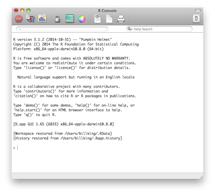
The window into which you type your commands is called the R Console. On the Mac and in Windows, this runs inside of a graphical user interface (GUI). In Linux, it runs in a terminal window. In the Mac and Windows version (but not in Linux) there are a few menus at the top of the window (in the menu bar on a Mac), and these are useful for a few things, mostly housekeeping tasks, but the commands that do your statistical work will be typed at the command prompt. The greater than sign (>) near the bottom of the window is the command prompt. You don't type this part--R supplies it. If the command extends onto two or more lines, this prompt will change to a plus sign (+), called the continuation prompt. Don't type the plus sign prompts either. With respect to that, an IMPORTANT NOTE: It will happen eventually (take my word for it!) that you will get stuck at a continuation prompt, and nothing you do will get you back to the command prompt. Don't panic! Press the Escape (Esc) key at the top left of your keyboard. That will abort the command currently being typed and bring you back to >. To see what that looks like, try this.
In R, as in many programming languages, comments start with pound symbols (#). Anything following a pound symbol is ignored by R and is there purely for the purpose of instruction or annotation. You don't need to type these bits. And did I mention that R is, in fact, a full featured programming language? You don't need to be intimidated by that. R has such a large number of built-in statistical functions that most people use it simply for interactive data analysis and graphics. It does mean, however, that R will be very picky about syntax. You will have to close all open parentheses, get your commas and quotes in the right places, and things like that. Annoying, I agree, and another common source of errors, but also very, very powerful! One thing you may find handy--commands can be copied and pasted into R. Don't copy the command prompts, however. Problem One: Weight Change in Anorexic Women Begin like this...
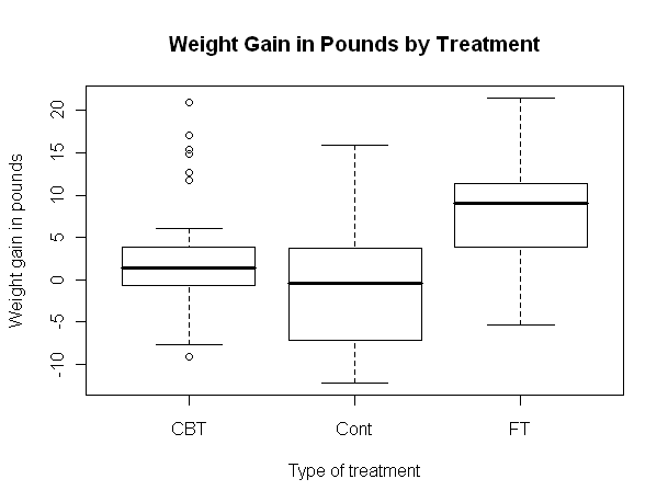
The second command loaded the "MASS" library, which contains the data set. The third command placed a copy of the data set "anorexia" into your workspace. The fourth command asked for a list of items stored in the workspace. The output produced by R is labeled [1]. The fifth command asked to see the structure of this data object. It is a data frame, which is a table-like object containing cases (or observations) in the rows and variables in the columns. There are 72 cases each measured on 3 variables. Those variables are Treat, a factor with 3 levels (CBT is cognitive behavioral therapy, Cont is a no-treatment control, and FT is family therapy), Prewt, a numeric variable (pretreatment weight in pounds), and Postwt, also a numeric variable (posttreatment weight in pounds). For more information, or to view the source for these data, request the help page by typing help(anorexia) at a command prompt. Help information will open in its own window in Windows and on the Mac. Close this window as you would any window on your system. In Linux, help information will open in the terminal. Press q (lower case Q) to return to the command prompt. We continue by examining the data. Don't worry about memorizing what all the
command do now. This is just for show. And remember, you don't have to type the
stuff after the # symbol.
If you're relatively new to computers (i.e., under the age of 50), here's something you will have to get used to about command line interfaces. Once something is printed to the screen, it's history, gone, done with. It will never be updated, changed or revised. ALL NEW INFORMATION OR CHANGES TO OLD INFORMATION WILL BE PRINTED OUT BELOW WHERE YOU TYPE A NEW COMMAND. So if you change something, you will have to issue a new command to see that change. What has already scrolled by is ancient history. Another thing you'll have to get used to is that when things go well in R,
R will often be silent. I.e., it will not tell you that it did what you told it
to do. You will have to ask it to show you. Here is an example.
Now let's draw a nice graph of the anorexia data. The graph will be drawn in a separate graphics window (called a "graphics device" in R-speak). If no such window is open, R will open one. If one is already open, R will use it and erase whatever graph is already there. So if you wanted a copy of that old graph, well, too late now! You should have saved it while you had the chance! You can manipulate this graphics window just like any other window on your system. You can move it around, resize it, and close it by clicking on the proper button. Closing the window will also erase the graph, so if you want to keep it, take steps to do so before writing over it or closing it. I'll tell you how to do this in a future tutorial. One thing I'll warn you about in advance though. When a new graphics device
window opens, it steals focus from the R Console. To type more commands, you'll
have to click in the R Console window with your mouse. (Wow! You get to use the
mouse!)
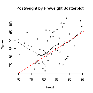
Now let's open a smaller graphics window and look at a scatterplot.
It appears the treatment effect is nonlinear, with lower preweight women
benefiting from treatment more than higher preweight women. In fact, it appears
that women with a preweight of 80 lbs. or more benefited hardly at all, on the
average. An analysis of variance is, therefore, suspect. Problem Two: Risk Factors Associated With Low Infant Birthweight We begin as before. You should not execute the library("MASS") command if you are still running the same R session. Try typing search(), and if you see "package:MASS" among the listed packages, it's already loaded. 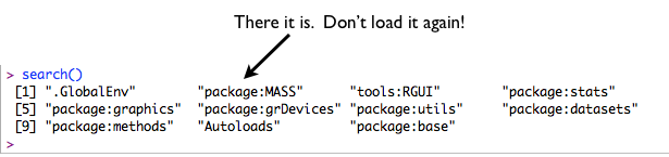
> library("MASS")            # Only if you have quit R since the last example.
> data(birthwt)              # Add this dataset to your workspace.
> ls()                       # List the contents of your workspace.
[1] "birthwt"
> str(birthwt)               # View the structure of the dataset.
'data.frame':   189 obs. of  10 variables:
 $ low  : int  0 0 0 0 0 0 0 0 0 0 ...
 $ age  : int  19 33 20 21 18 21 22 17 29 26 ...
 $ lwt  : int  182 155 105 108 107 124 118 103 123 113 ...
 $ race : int  2 3 1 1 1 3 1 3 1 1 ...
 $ smoke: int  0 0 1 1 1 0 0 0 1 1 ...
 $ ptl  : int  0 0 0 0 0 0 0 0 0 0 ...
 $ ht   : int  0 0 0 0 0 0 0 0 0 0 ...
 $ ui   : int  1 0 0 1 1 0 0 0 0 0 ...
 $ ftv  : int  0 3 1 2 0 0 1 1 1 0 ...
 $ bwt  : int  2523 2551 2557 2594 2600 2622 2637 2637 2663 2665 ...
I will begin by recoding some of the variables to make them factors. This could
have been done when the data set was first prepared, but it wasn't. If you've
jumped the gun and have already attached the dataframe, detach it. NEVER modify
an attached dataframe. (It's not against the law, and it really doesn't even hurt
anything, but you'll end up becoming terribly confused! Because...? Mods to data
frames don't affect the attached copy, which is what you'll be working from.)
> ### low: birthwt below 2.5 kg, 0=no, 1=yes; we will leave this as is
> ### age: age of mother in years; a numeric variable; no need to recode
> ### lwt: weight of mother in pounds at last menstrual period; numeric; no need to recode
> ### race: R thinks this is an integer, so we want to (very carefully!!) recode
> value.labels = c("white","black","other")
> birthwt$race = factor(birthwt$race, labels=value.labels)
> ### Note: birthwt$race means the race variable inside the birthwt data frame
> ### smoke: smoking status during pregnancy (0="no", 1="yes"); also needs recoding
> value.labels = c("no","yes")         # this could be done in one step, if you're brave enough!
> birthwt$smoke = factor(birthwt$smoke, labels=value.labels)
> ### ptl: number of previous premature labors; no need to recode
> ### ht: history of hypertension (0="no", 1="yes")
> birthwt$ht = factor(birthwt$ht, labels=value.labels)
> ### ui: presence of uterine irritability (0="no", 1="yes")
> birthwt$ui = factor(birthwt$ui, labels=value.labels)
> ### ftv: number of physician visits during first trimester
> ### bwt: birth weight of baby in grams; change to kilograms
> birthwt$bwt = birthwt$bwt / 1000
> summary(birthwt)
      low              age             lwt           race    smoke
 Min.   :0.0000   Min.   :14.00   Min.   : 80.0   white:96   no :115
 1st Qu.:0.0000   1st Qu.:19.00   1st Qu.:110.0   black:26   yes: 74
 Median :0.0000   Median :23.00   Median :121.0   other:67
 Mean   :0.3122   Mean   :23.24   Mean   :129.8
 3rd Qu.:1.0000   3rd Qu.:26.00   3rd Qu.:140.0
 Max.   :1.0000   Max.   :45.00   Max.   :250.0
      ptl           ht        ui           ftv              bwt
 Min.   :0.0000   no :177   no :161   Min.   :0.0000   Min.   :0.709
 1st Qu.:0.0000   yes: 12   yes: 28   1st Qu.:0.0000   1st Qu.:2.414
 Median :0.0000                       Median :0.0000   Median :2.977
 Mean   :0.1958                       Mean   :0.7937   Mean   :2.945
 3rd Qu.:0.0000                       3rd Qu.:1.0000   3rd Qu.:3.487
 Max.   :3.0000                       Max.   :6.0000   Max.   :4.990
Notice that summary is a very intelligent command. It knows to summarize
numbers as numbers and factors as factors. It will get even smarter in the
future. Let's crosstabulate some of the categorical variables (factors).
> attach(birthwt)                 # Makes the variables inside birthwt visible without the $ thing.
> table(smoke, low)               # Hence, we don't need to type birthwt$smoke, etc.
     low
smoke  0  1
  no  86 29
  yes 44 30
>                                 # Inserting a blank line now and then makes things easier to read.
> xtabs(~ smoke + low)            # An alternate form that does the same thing.
     low
smoke  0  1
  no  86 29
  yes 44 30
>
> table(smoke, race)              # Remember, the space after the comma is optional.
     race
smoke white black other
  no     44    16    55
  yes    52    10    12
>
> table(smoke,ht,ui,low)          # A four-dimensional contingency table.
, , ui = no, low = 0

     ht
smoke no yes
  no  75   3
  yes 36   2

, , ui = yes, low = 0

     ht
smoke no yes
  no   8   0
  yes  6   0

, , ui = no, low = 1

     ht
smoke no yes
  no  18   4
  yes 20   3

, , ui = yes, low = 1

     ht
smoke no yes
  no   7   0
  yes  7   0

> big.table = table(smoke,ht,ui,low)        # Store output rather than printing it.
> ftable(big.table)                         # A more convenient way to view this.
              low  0  1
smoke ht  ui
no    no  no      75 18
          yes      8  7
      yes no       3  4
          yes      0  0
yes   no  no      36 20
          yes      6  7
      yes no       2  3
          yes      0  0

> flat.table = ftable(big.table)            # Store output so we can work with it.
> prop.table(flat.table, 1)                 # As proportions rather than raw freqs.
              low         0         1
smoke ht  ui
no    no  no      0.8064516 0.1935484
          yes     0.5333333 0.4666667
      yes no      0.4285714 0.5714286
          yes           NaN       NaN
yes   no  no      0.6428571 0.3571429
          yes     0.4615385 0.5384615
      yes no      0.4000000 0.6000000
          yes           NaN       NaN
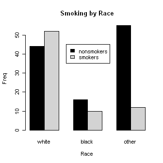 Let's look at smoking by race. Some of these commands are long, so I broke them
in the middle by hitting Enter and continuing on the next line. (On a Mac
you'll have to erase the close parenthesis first.) Remember not to
type the + signs, as R will supply them. And spacing is optional. I added some
spacing to make the command easier to read. Watch your commas and quotes, too.
One missed or misplaced comma will make the whole command wrong!
Let's look at smoking by race. Some of these commands are long, so I broke them
in the middle by hitting Enter and continuing on the next line. (On a Mac
you'll have to erase the close parenthesis first.) Remember not to
type the + signs, as R will supply them. And spacing is optional. I added some
spacing to make the command easier to read. Watch your commas and quotes, too.
One missed or misplaced comma will make the whole command wrong!
> smoke.by.race = table(smoke, race)
> barplot(smoke.by.race, beside=T,
+         main="Smoking by Race",
+         ylab="Freq", xlab="Race",
+         col=c("black","lightgray"))
> legend(x=3.5, y=45, legend=c("nonsmokers","smokers"),
+         fill=c("black","lightgray"))
> results = chisq.test(smoke.by.race)
> results

        Pearson's Chi-squared test

data:  smoke.by.race
X-squared = 21.779, df = 2, p-value = 1.865e-05

> results$expected                          # View the expected frequencies.
     race
smoke   white    black    other
  no  58.4127 15.82011 40.76720
  yes 37.5873 10.17989 26.23280
> results$residuals                         # View the (standardized) residuals in each cell.
     race
smoke       white       black       other
  no  -1.88578277  0.04522852  2.22912825
  yes  2.35084895 -0.05638265 -2.77886927
Are any of the factors related to low birthweight? We'll find out by using
logistic regression, an advanced technique incorporated into the default R
packages you get at download.
> glm.out = glm(low ~ race + smoke + ht + ui, family=binomial(logit))
> summary(glm.out)

Call:
glm(formula = low ~ race + smoke + ht + ui, family = binomial(logit))

Deviance Residuals:
    Min       1Q   Median       3Q      Max
-1.6618  -0.7922  -0.4825   1.1413   2.1016

Coefficients:
            Estimate Std. Error z value Pr(>|z|)
(Intercept)  -2.0919     0.3800  -5.505 3.69e-08 ***
raceblack     1.0638     0.4990   2.132  0.03301 *
raceother     1.0834     0.4131   2.622  0.00873 **
smokeyes      1.0940     0.3797   2.881  0.00397 **
htyes         1.3594     0.6297   2.159  0.03087 *
uiyes         1.0059     0.4385   2.294  0.02179 *
---
Signif. codes:  0 '***' 0.001 '**' 0.01 '*' 0.05 '.' 0.1 ' ' 1

(Dispersion parameter for binomial family taken to be 1)

    Null deviance: 234.67  on 188  degrees of freedom
Residual deviance: 211.17  on 183  degrees of freedom
AIC: 223.17

Number of Fisher Scoring iterations: 4
Apparently they all are! Don't forget to clean up your workspace and search
path.
> detach(birthwt)                 ### Always detach after you attach!
> ls()                            # List contents of workspace. Or you could do this from a menu.
[1] "big.table"     "birthwt"       "flat.table"    "glm.out"
[5] "results"       "smoke.by.race"
> rm(list=ls())                   # Completely clear the workspace. You can also do this from a menu.
>ls()
character(0)
Notice that when I was naming things, I did not put spaces or dashes in those names. R wouldn't like that! Use a period instead. Notice also that the chisq.test( ) and glm( ) commands produced no output when they were executed, because that output was stored in results and glm.out, respectively. We then had to ask to see the results, in one case by using summary(glm.out). This is typically how R works. Problem Three: Some Factors Associated With Car Insurance Claims As before, don't execute the library()
command if you are still in the same active R session (MASS still in the search
path).
There is no replication within the cells, so a fully crossed 3-way ANOVA
would leave us without an error term. Examination of the data reveals an
apparent absence of interactions. So we will request a 3-way ANOVA without
testing the interactions.
My advice would be not to do something so silly as to use greater than, less than, and minus signs in your group names. Just a thought! But notice even when something so silly as mathematical operators are included in group names, R can handle it if you're careful. I would also not take those results at face value, as an examination of the model assumptions reveals heterogeneity of variance and nonnormality. Perhaps a transform of the response could fix that. 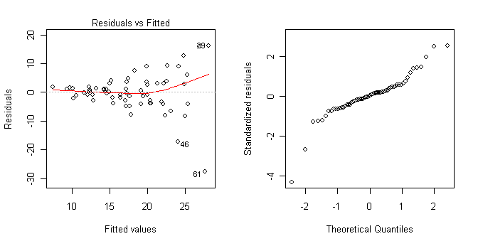
Yes, those graphs were also created in R. They show clearly that the homogeneity of variance and normal distribution assumptions have been violated. > ls() [1] "aov.out" "Insurance" > rm(list=ls()) ### Clean up the mess we've made.There is no need to detach Insurance because it was never attached. Check the search path to confirm this if you don't remember. And by the way, deleting it does not detach it. Problem Four: Some Cars Sold In the United States in 1993
> library("MASS")                      ### Don't do this if it's already done.
> ### If you accidentally attach something twice, no harm no foul.
> ### Just detach it once.
> data(Cars93)
> str(Cars93)
'data.frame':   93 obs. of  27 variables:
 $ Manufacturer      : Factor w/ 32 levels "Acura","Audi",..: 1 1 2 2 3 4 4 4 4 5 ...
 $ Model             : Factor w/ 93 levels "100","190E","240",..: 49 56 9 1 6 24 54 74 73 35 ...
 $ Type              : Factor w/ 6 levels "Compact","Large",..: 4 3 1 3 3 3 2 2 3 2 ...
 $ Min.Price         : num  12.9 29.2 25.9 30.8 23.7 14.2 19.9 22.6 26.3 33 ...
 $ Price             : num  15.9 33.9 29.1 37.7 30 15.7 20.8 23.7 26.3 34.7 ...
 $ Max.Price         : num  18.8 38.7 32.3 44.6 36.2 17.3 21.7 24.9 26.3 36.3 ...
 $ MPG.city          : int  25 18 20 19 22 22 19 16 19 16 ...
 $ MPG.highway       : int  31 25 26 26 30 31 28 25 27 25 ...
 $ AirBags           : Factor w/ 3 levels "Driver & Passenger",..: 3 1 2 1 2 2 2 2 2 2 ...
 $ DriveTrain        : Factor w/ 3 levels "4WD","Front",..: 2 2 2 2 3 2 2 3 2 2 ...
 $ Cylinders         : Factor w/ 6 levels "3","4","5","6",..: 2 4 4 4 2 2 4 4 4 5 ...
 $ EngineSize        : num  1.8 3.2 2.8 2.8 3.5 2.2 3.8 5.7 3.8 4.9 ...
 $ Horsepower        : int  140 200 172 172 208 110 170 180 170 200 ...
 $ RPM               : int  6300 5500 5500 5500 5700 5200 4800 4000 4800 4100 ...
 $ Rev.per.mile      : int  2890 2335 2280 2535 2545 2565 1570 1320 1690 1510 ...
 $ Man.trans.avail   : Factor w/ 2 levels "No","Yes": 2 2 2 2 2 1 1 1 1 1 ...
 $ Fuel.tank.capacity: num  13.2 18 16.9 21.1 21.1 16.4 18 23 18.8 18 ...
 $ Passengers        : int  5 5 5 6 4 6 6 6 5 6 ...
 $ Length            : int  177 195 180 193 186 189 200 216 198 206 ...
 $ Wheelbase         : int  102 115 102 106 109 105 111 116 108 114 ...
 $ Width             : int  68 71 67 70 69 69 74 78 73 73 ...
 $ Turn.circle       : int  37 38 37 37 39 41 42 45 41 43 ...
 $ Rear.seat.room    : num  26.5 30 28 31 27 28 30.5 30.5 26.5 35 ...
 $ Luggage.room      : int  11 15 14 17 13 16 17 21 14 18 ...
 $ Weight            : int  2705 3560 3375 3405 3640 2880 3470 4105 3495 3620 ...
 $ Origin            : Factor w/ 2 levels "USA","non-USA": 2 2 2 2 2 1 1 1 1 1 ...
 $ Make              : Factor w/ 93 levels "Acura Integra",..: 1 2 4 3 5 6 7 9 8 10 ...
What would be interesting to look at here?
revised 2016 January 14 |