
| Table of Contents
| Function Reference
| Function Finder
| R Project |
SIMPLE LINEAR CORRELATION AND REGRESSION
Correlation
Correlation is used to test for a relationship between two numeric
variables or two ranked (ordinal) variables. In this tutorial, we assume the
relationship (if any) is linear.
To demonstrate, we will begin with a data set called "cats" from the "MASS"
library, which contains information on various anatomical features of house
cats.
> library("MASS")
> data(cats)
> str(cats)
'data.frame':   144 obs. of  3 variables:
 $ Sex: Factor w/ 2 levels "F","M": 1 1 1 1 1 1 1 1 1 1 ...
 $ Bwt: num  2 2 2 2.1 2.1 2.1 2.1 2.1 2.1 2.1 ...
 $ Hwt: num  7 7.4 9.5 7.2 7.3 7.6 8.1 8.2 8.3 8.5 ...
> summary(cats)
 Sex         Bwt             Hwt
 F:47   Min.   :2.000   Min.   : 6.30
 M:97   1st Qu.:2.300   1st Qu.: 8.95
        Median :2.700   Median :10.10
        Mean   :2.724   Mean   :10.63
        3rd Qu.:3.025   3rd Qu.:12.12
        Max.   :3.900   Max.   :20.50
"Bwt" is the body weight in kilograms, "Hwt" is the heart weight in grams, and
"Sex" should be obvious. There are no missing values in any of the variables, so
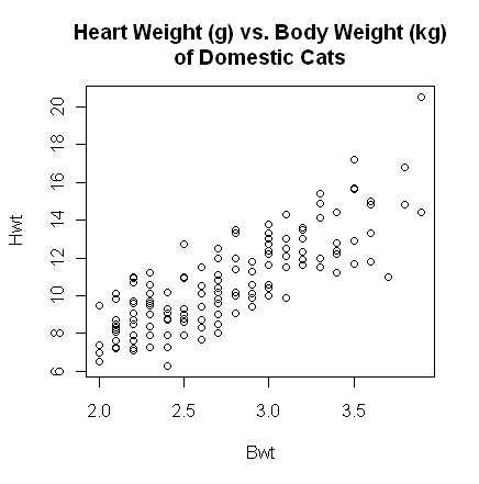
we are ready to begin by looking at a scatterplot.
> with(cats, plot(Bwt, Hwt))
> title(main="Heart Weight (g) vs. Body Weight (kg)\nof Domestic Cats")
 The plot() function gives a scatterplot whenever
you feed it two numeric
variables. The first variable listed will be plotted on the horizontal axis. A
formula interface can also be used, in which case the response variable should
come before the tilde and the variable to be plotted on the horizontal axis
after. (Close the graphics window before doing this, because the output will
look exactly the same.)
The plot() function gives a scatterplot whenever
you feed it two numeric
variables. The first variable listed will be plotted on the horizontal axis. A
formula interface can also be used, in which case the response variable should
come before the tilde and the variable to be plotted on the horizontal axis
after. (Close the graphics window before doing this, because the output will
look exactly the same.)
> with(cats, plot(Hwt ~ Bwt))     # or...
> plot(Hwt ~ Bwt, data=cats)
The scatterplot shows a fairly strong and reasonably linear relationship between
the two variables. A Pearson product-moment correlation coefficient can be
calculated using the cor() function (which will fail
if there are missing values).
> with(cats, cor(Bwt, Hwt))
[1] 0.8041274
> with(cats, cor(Bwt, Hwt))^2
[1] 0.6466209
Pearson's r = .804 indicates a strong positive relationship. To get the
coefficient of determination, I just hit the up arrow key to recall the
previous command to the command line and added "^2" on the end to square it. If
a test of significance is required, this is also easily enough done using the
cor.test() function. The function does a t-test,
a 95% confidence
interval for the population correlation (use "conf.level=" to change the
confidence level), and reports the value of the sample statistic. The
alternative hypothesis can be set to "two.sided" (the default), "less", or
"greater". (Meaning less than 0 or greater than 0 in most cases.)
> with(cats, cor.test(Bwt, Hwt))       # cor.test(~Bwt + Hwt, data=cats) also works

        Pearson's product-moment correlation

data:  Bwt and Hwt
t = 16.1194, df = 142, p-value < 2.2e-16
alternative hypothesis: true correlation is not equal to 0
95 percent confidence interval:
 0.7375682 0.8552122
sample estimates:
      cor
0.8041274
Since we would expect a positive correlation here, we might have set the
alternative to "greater".
> with(cats, cor.test(Bwt, Hwt, alternative="greater", conf.level=.8))

        Pearson's product-moment correlation

data:  Bwt and Hwt
t = 16.1194, df = 142, p-value < 2.2e-16
alternative hypothesis: true correlation is greater than 0
80 percent confidence interval:
 0.7776141 1.0000000
sample estimates:
      cor
0.8041274
There is also a formula interface for cor.test(),
but it's tricky. Both variables should be listed after the tilde. (Order of the
variables doesn't matter in either the cor() or the
cor.test() function.)
> cor.test(~ Bwt + Hwt, data=cats) # output not shown
Using the formula interface makes it easy to subset the data by rows of the
data frame.
> cor.test(~Bwt + Hwt, data=cats, subset=(Sex=="F"))

	Pearson's product-moment correlation

data:  Bwt and Hwt
t = 4.2152, df = 45, p-value = 0.0001186
alternative hypothesis: true correlation is not equal to 0
95 percent confidence interval:
 0.2890452 0.7106399
sample estimates:
      cor
0.5320497
The "subset=" option is not available unless you use the formula interface.
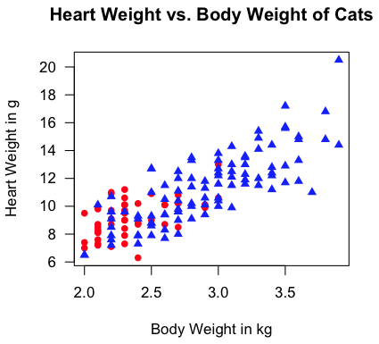
For a more revealing scatterplot, try this.
> with(cats, plot(Bwt, Hwt, type="n", las=1, xlab="Body Weight in kg",
+                 ylab="Heart Weight in g",
+                 main="Heart Weight vs. Body Weight of Cats"))
> with(cats, points(Bwt[Sex=="F"], Hwt[Sex=="F"], pch=16, col="red"))
> with(cats, points(Bwt[Sex=="M"], Hwt[Sex=="M"], pch=17, col="blue"))
"Aw, man! I'm not gonna type all that!" Fine! I don't blame you (much).
Copy those lines from this webpage and then paste them into a script window
(File > New Script in Windows or File > New Document on a Mac). Erase the
command prompts, and then execute. But if you type it yourself, you get to
see what happens step by step. (See the tutorial on
scripts for details on how to use them.)
Correlation and Covariance Matrices
If a data frame (or other table-like object) contains more than two numeric
variables, then the cor() function will result in
a correlation matrix.
> rm(cats)                             # if you haven't already
> data(cement)                         # also in the MASS library
> str(cement)
'data.frame':   13 obs. of  5 variables:
 $ x1: int  7 1 11 11 7 11 3 1 2 21 ...
 $ x2: int  26 29 56 31 52 55 71 31 54 47 ...
 $ x3: int  6 15 8 8 6 9 17 22 18 4 ...
 $ x4: int  60 52 20 47 33 22 6 44 22 26 ...
 $ y : num   78.5  74.3 104.3  87.6  95.9 ...
> cor(cement)                          # fails if there are missing values
           x1         x2          x3          x4          y
x1  1.0000000  0.2285795 -0.82413376 -0.24544511  0.7307175
x2  0.2285795  1.0000000 -0.13924238 -0.97295500  0.8162526
x3 -0.8241338 -0.1392424  1.00000000  0.02953700 -0.5346707
x4 -0.2454451 -0.9729550  0.02953700  1.00000000 -0.8213050
y   0.7307175  0.8162526 -0.53467068 -0.82130504  1.0000000
If you prefer a covariance matrix, use cov().
> cov(cement)                          # also fails if there are missing values
          x1         x2         x3          x4          y
x1  34.60256   20.92308 -31.051282  -24.166667   64.66346
x2  20.92308  242.14103 -13.878205 -253.416667  191.07949
x3 -31.05128  -13.87821  41.025641    3.166667  -51.51923
x4 -24.16667 -253.41667   3.166667  280.166667 -206.80833
y   64.66346  191.07949 -51.519231 -206.808333  226.31359
If you have a covariance matrix and want a correlation matrix...
> cov.matr = cov(cement)
> cov2cor(cov.matr)
           x1         x2          x3          x4          y
x1  1.0000000  0.2285795 -0.82413376 -0.24544511  0.7307175
x2  0.2285795  1.0000000 -0.13924238 -0.97295500  0.8162526
x3 -0.8241338 -0.1392424  1.00000000  0.02953700 -0.5346707
x4 -0.2454451 -0.9729550  0.02953700  1.00000000 -0.8213050
y   0.7307175  0.8162526 -0.53467068 -0.82130504  1.0000000
If you want a visual representation of the correlation matrix (i.e., a
scatterplot matrix)...
> pairs(cement)
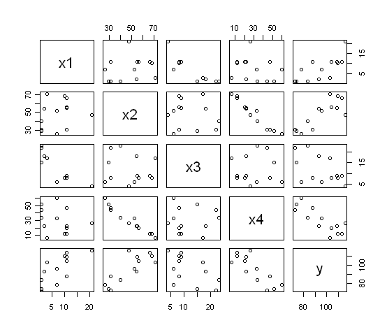 The command plot(cement) would also have done the
same thing.
The command plot(cement) would also have done the
same thing.
Correlations for Ranked Data
If the data are ordinal rather than true numerical measures, or have been
converted to ranks to fix some problem with distribution or curvilinearity, then
R can calculate a Spearman rho coefficient or a Kendall tau coefficient. Suppose
we have two athletic coaches ranking players by skill.
> ls()
[1] "cement"   "cov.matr"
> rm(cement, cov.matr)                      # clean up first
> coach1 = c(1,2,3,4,5,6,7,8,9,10)
> coach2 = c(4,8,1,5,9,2,10,7,3,6)
> cor(coach1, coach2, method="spearman")    # do not capitalize "spearman"
[1] 0.1272727
> cor.test(coach1, coach2, method="spearman")

        Spearman's rank correlation rho

data:  coach1 and coach2
S = 144, p-value = 0.72
alternative hypothesis: true rho is not equal to 0
sample estimates:
      rho
0.1272727

> cor(coach1, coach2, method="kendall")
[1] 0.1111111
> cor.test(coach1, coach2, method="kendall")

        Kendall's rank correlation tau

data:  coach1 and coach2
T = 25, p-value = 0.7275
alternative hypothesis: true tau is not equal to 0
sample estimates:
      tau
0.1111111

> ls()
[1] "coach1" "coach2"
> rm(coach1,coach2)                         # clean up again
I will not get into the debate over which of these rank correlations is
better! You can also use the "alternative=" option here to set a directional
test.
How To Get These Functions To Work If There Are Missing Values
As noted, missing values cause these functions to cough up a hair ball.
Here's how to get around it. We'll use the cats data again, but will insert
a few missings.
> data(cats)
> cats[12,2] = NA
> cats[101,3] = NA
> cats[132,2:3] = NA
> summary(cats)
 Sex         Bwt             Hwt
 F:47   Min.   :2.000   Min.   : 6.30
 M:97   1st Qu.:2.300   1st Qu.: 8.85
        Median :2.700   Median :10.10
        Mean   :2.723   Mean   :10.62
        3rd Qu.:3.000   3rd Qu.:12.07
        Max.   :3.900   Max.   :20.50
        NA's   :2       NA's   :2
> with(cats, cor(Bwt, Hwt))
[1] NA
Okay, it's not a hair ball, it's an NA. Easier on your carpet! Let's see what
works and what doesn't.
> with(cats, cor(Bwt, Hwt))            # fails
> with(cats, cov(Bwt, Hwt))            # fails
> with(cats, cor.test(Bwt, Hwt))       # works! (I didn't think it would.)
> with(cats, plot(Bwt, Hwt))           # works
To get cor() and cov()
to work with missing values, you set the "use=" option. Possible values are
"everything", "all.obs" (not sure what the difference is there), "complete.obs"
(deletes cases with any missing values from the computation even if there are
no missings in the two variables that are currently being computed with),
"na.or.complete" (pretty much the same), and "pairwise.complete.obs" (all
complete pairs of the two variables currently being considered are used).
> with(cats, cor(Bwt, Hwt, use="pairwise"))
[1] 0.8066677
You only need to type enough of the option value that R can recognize it (thank
goodness in this case).
Simple Linear Regression
There is little question that R was written with regression analysis in mind!
The number of functions and add-on packages devoted to regression analysis of
one kind or another is staggering! We will only scratch the surface in
this tutorial.
Let's go back to our kitty cat data.
> rm(cats)                             # get rid of the messed up version
> data(cats)                           # still in the "MASS" library
Simple (as well as multiple) linear regression is done using the lm()
function. This function requires a formula interface, and for simple regression
the formula takes the form DV ~ IV, which should be read something
like "DV as a function of IV" or "DV as modeled by IV" or "DV as predicted by
IV", etc. It's critical to remember that the DV or response variable must come
before the tilde and IV or explanatory variables after. Getting the regression
equation for our "cats" is simple enough.
> lm(Hwt ~ Bwt, data=cats)

Call:
lm(formula = Hwt ~ Bwt, data = cats)

Coefficients:
(Intercept)          Bwt
    -0.3567       4.0341
So the regression equation is: Hwt-hat = 4.0341 (Bwt) - 0.3567. A better idea
is to store the output into a data object and then to extract information from
that with various extractor functions.
> lm.out = lm(Hwt ~ Bwt, data=cats)    # name the output anything you like
> lm.out                               # gives the default output

Call:
lm(formula = Hwt ~ Bwt, data = cats)

Coefficients:
(Intercept)          Bwt
    -0.3567       4.0341

> summary(lm.out)                      # gives a lot more info

Call:
lm(formula = Hwt ~ Bwt, data = cats)

Residuals:
    Min      1Q  Median      3Q     Max
-3.5694 -0.9634 -0.0921  1.0426  5.1238

Coefficients:
            Estimate Std. Error t value Pr(>|t|)
(Intercept)  -0.3567     0.6923  -0.515    0.607
Bwt           4.0341     0.2503  16.119   <2e-16 ***
---
Signif. codes:  0 '***' 0.001 '**' 0.01 '*' 0.05 '.' 0.1 ' ' 1

Residual standard error: 1.452 on 142 degrees of freedom
Multiple R-squared:  0.6466,	Adjusted R-squared:  0.6441
F-statistic: 259.8 on 1 and 142 DF,  p-value: < 2.2e-16
Personally, I don't like those significance stars, so I'm going to turn them
off. (It'll also save me from having to erase the smart quotes from the R
output and replace them with ordinary sane quotes. Really, R people? Smart
quotes?!)
> options(show.signif.stars=F)
> anova(lm.out)                        # shows an ANOVA table
Analysis of Variance Table

Response: Hwt
           Df Sum Sq Mean Sq F value    Pr(>F)
Bwt         1 548.09  548.09  259.83 < 2.2e-16
Residuals 142 299.53    2.11
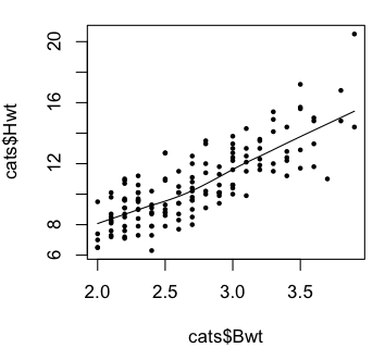
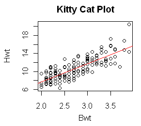 With the output saved in a data object, plotting the regression line on a
pre-existing scatterplot is a cinch.
With the output saved in a data object, plotting the regression line on a
pre-existing scatterplot is a cinch.
> plot(Hwt ~ Bwt, data=cats, main="Kitty Cat Plot")
> abline(lm.out, col="red")
And I'll make the regression line red just because I can!
Various regression diagnostics are also available. These will be discussed
more completely in future tutorials, but for now, a graphic display of how good
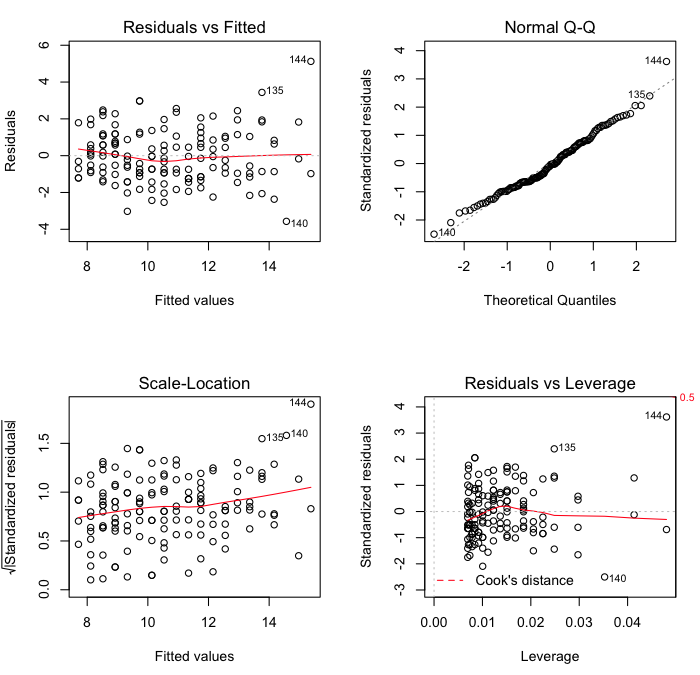
the model fit is can be achieved as follows.
> par(mfrow=c(2,2))          # partition the graphics device
> plot(lm.out)
 The first of these commands sets the parameters of the graphics device. If your
graphics output window was closed, you probably noticed it opening when this
command was issued. Specifically, the command partitioned the graphics window
into four parts, two rows by two columns, so four graphs could be plotted in
one window. The graphics window will retain this structure until you either
close it, in which case it will return to its default next time it opens, or
you reset it with par(mfrow=c(1,1)). If you do not
partition the graphics window first, then each diagnostic plot will print out
in a separate window. R will give you a cryptic message, "Waiting to confirm
page change...", in the console before each graph is displayed. This means hit
the Enter key to display the next graph. The second command, plot(), then does the actual plotting.
The first of these commands sets the parameters of the graphics device. If your
graphics output window was closed, you probably noticed it opening when this
command was issued. Specifically, the command partitioned the graphics window
into four parts, two rows by two columns, so four graphs could be plotted in
one window. The graphics window will retain this structure until you either
close it, in which case it will return to its default next time it opens, or
you reset it with par(mfrow=c(1,1)). If you do not
partition the graphics window first, then each diagnostic plot will print out
in a separate window. R will give you a cryptic message, "Waiting to confirm
page change...", in the console before each graph is displayed. This means hit
the Enter key to display the next graph. The second command, plot(), then does the actual plotting.
The first plot is a standard residual plot showing residuals against fitted
values. Points that tend towards being outliers are labeled. If any pattern is
apparent in the points on this plot, then the linear model may not be the
appropriate one. The second plot is a normal quantile plot of the residuals. We
like to see our residuals normally distributed. Don't we? The last plot shows
residuals vs. leverage. Labeled points on this plot represent cases we may want
to investigate as possibly having undue influence on the regression
relationship. Case 144 is one perhaps worth taking a look at.
> cats[144,]
    Sex Bwt  Hwt
144   M 3.9 20.5
> lm.out$fitted[144]
     144
15.37618
> lm.out$residuals[144]
     144
5.123818
This cat had the largest body weight and the largest heart weight in the data
set. (See the summary table at the top of this tutorial.) The observed value of
"Hwt" was 20.5g, but the fitted value was only 15.4g, giving a residual of
5.1g. The residual standard error (from the model output above) was 1.452, so
converting this to a standardized residual gives 5.124/1.452 = 3.53, a substantial
value to say the least! A commonly used measure of influence is Cook's Distance,
which can be visualized for all the cases in the model as follows.
> par(mfrow=c(1,1))                    # if you haven't already done this
> plot(cooks.distance(lm.out))         # also try plot(lm.out, 4)
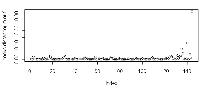 As we can see, case 144 tops the charts.
There are a number of ways to proceed. One is to look at the regression
coefficients without the outlying point in the model.
> lm.without144 = lm(Hwt ~ Bwt, data=cats, subset=(Hwt<20.5))
> ### another way to do this is lm(Hwt ~ Bwt, data=cats[-144,])
> lm.without144

Call:
lm(formula = Hwt ~ Bwt, subset = (Hwt < 20.5))

Coefficients:
(Intercept)          Bwt
      0.118        3.846
Another is to use a procedure that is robust in the face of outlying points.
> rlm(Hwt ~ Bwt, data=cats)
Call:
rlm(formula = Hwt ~ Bwt)
Converged in 5 iterations

Coefficients:
(Intercept)         Bwt
 -0.1361777   3.9380535

Degrees of freedom: 144 total; 142 residual
Scale estimate: 1.52
See the help page on rlm() for the details of
what this function does.
Lowess
Lowess stands for locally weighted scatterplot smoothing. It is a
nonparametric method for drawing a smooth curve through a scatterplot. There
are at least two ways to produce such a plot in R.
> plot(Hwt ~ Bwt, data=cats)
> lines(lowess(cats$Hwt ~ cats$Bwt), col="red")
> ### the lowess() function will take a formula interface but will not use
> ### the data= option; an oversight in the programming, I suspect
>
> ### the other method is (close the graphics device first)...
>
> scatter.smooth(cats$Hwt ~ cats$Bwt)       # same programming flaw here
> scatter.smooth(cats$Hwt ~ cats$Bwt, pch=16, cex=.6)
 The plots indicate we were on the right track with our linear model.
revised 2016 February 15
| Table of Contents
| Function Reference
| Function Finder
| R Project |
|