SAVING AND LOADING OBJECTS IN R

The Workspace and History

You've probably noticed already, when you start and quit R, you see something like this.

R version 3.1.2 (2014-10-31) -- "Pumpkin Helmet"
Copyright (C) 2014 The R Foundation for Statistical Computing

.
.
.

[Workspace restored from /Users/billking/.RData]
[History restored from /Users/billking/.Rapp.history]

> quit()
Save workspace image? [y/n/c]:

Your workspace, remember, consists of all the data objects you've created or loaded during your R session (and perhaps a few other things as well). When R asks if you want to save your workspace image before quitting, and you say "no", all of the NEW stuff you've created goes away--forever. If you say "yes", then a file called ".RData" is written to your working directory. The next time you start R in this directory, that workspace and all its data objects will be restored.

This is extremely convenient for people who are running R in a terminal, such as the terminal.app in OS X or a Linux terminal. Those people can devote a working directory to each problem they are working on, and when they start R, they can simply change to that directory FIRST (before starting R), and R will open with that directory as the working directory and restore the workspace from there. It's not so convenient for people who are running R in Windows or in the Mac R GUI console, in which case R will always start in the same default working directory, IF you start it from the Dock or Desktop shortcut. In Windows XP that will be "My Documents". In Windows Vista and (I suspect) Windows 7/8/10, it is the user's home directory. On the Mac and in Linux it will be the user's home directory.

(NOTE: If you don't know what your home directory is, then start R and use getwd(). If you want R to start somewhere else, there are several ways to do that, and differ somewhat in Windows vs. Mac. Google "default working directory R." And be prepared for more info on this than you probably cared to see!)

(STUDENTS: If you are working in one of your university's computer labs, heaven help you! Due to various "security measures" typically in place on these machines, you may have trouble running R at all! Here at CCU, if you are working in Windows, it is ALWAYS necessary to start R from the desktop shortcut. That makes the Desktop your working directory-- don't ask me why! You should have read/write privileges to the Desktop, so R should work for you. You should create your "Rspace" folder on the Desktop. If you're working on one of the university's Macs, well, it's different!)

When R opens, it will load the workspace file (".RData") if there is one, and it will also load the history file (".Rhistory") if there is one. If you then change your working directory, to "Rspace" let's say, R will bring along the already loaded workspace and history files, but it WILL NOT load any such files you've stored in "Rspace".

(ANOTHER NOTE: The history file is a list of commands entered during previous R sessions. I never work with the history file and don't claim to understand it. It appears to have gotten much more confusing in the 5.5 years since I last revised this tutorial, and quite frankly I'm in no mood to try to untangle it. Therefore, I will make no further mention of it. Type help(history) at the command prompt for more info.)

Let's say you have the following work habits. You open R, you change to "Rspace", you do your R business, you quit R and opt to save the workspace. The next time you start R, your previously created data objects are nowhere to be seen, even after you change the working directory to "Rspace". Here's how to retrieve them. First, you may want to get rid of any workspace items R has dragged along from the default working directory. That can be done with the rm() function. Then you can load the previously saved workspace (and presumably the history file if so desired) like this.

> ls()                                 # This is my default workspace from My Documents (WinXP).
[1] "age.out"       "m.ex"          "m.ex.minussex" "outcome.out"  
[5] "respiratory"   "seizure"       "visit.matrix"
> setwd("Rspace")                      # First change, if you haven't already.
> rm(list=ls())                        # Delete the default workspace.
> load(".RData")                       # Load a previously saved workspace.
> loadhistory()                        # Load a previously saved history file.
> ls()
[1] "my.data"

If you change the workspace, say by removing "my.data", but then don't save it when you quit or before you change the working directory, "my.data" will still be there when you come back next time. It's like any other document. If you make changes to a word processing document, but then don't save it, or save it to a new folder/directory, then the same old version will be there (in the old directory) next time you start up. The difference is that R won't nag you about saving changes. It will ask you if you want to save your workspace, changes or no, and if you don't, well then fine with R! (R Studio appears to be different. It will ask you to save the workspace only when changes have been made.)

Another difference between R and word processors is that R won't remember where you got the document from. When you quit and save the workspace, it will be saved in the current working directory. Period! (Unless you tell it to do other wise by using a complete or relative pathname.)

The rm() function modifies the workspace, but NOT the workspace image file (".RData"). If you remove "my.data" and save the workspace when you quit, "my.data" will be gone because the new workspace image (.RData file) will overwrite the old one. If you change working directories and then load ".RData" in the new directory, R will ADD it to whatever you've brought with you from the previous working directory. If you don't want that, be sure to clear the old workspace before loading the new one.

If your work sessions are long, it's a good idea to save a workspace image once in awhile, because this image is held in RAM. That means if the power goes out, it's gone. You can save a workspace image at any time by doing this, which has the same effect as choosing "Yes, please save my workspace" when you quit.

> save.image()                         # Save an .RData file.
> savehistory()                        # Save an .Rhistory file.

> save.image(file="workspace21.RData")

> load(file="workspace21.RData")

It takes awhile to get used to how the workspace and history files work, when they are saved, when the existing ones are modified, and so on, but it's really quite logical. R is a good old fashioned command line program. It does not do anything that you don't tell it to do. This is one of its BEST features as far as I'm concerned! If you want it to do things automatically upon startup and shutdown, there are scripts you can modify, but that is beyond the scope of this tutorial.

Scripts

This section has been removed from this tutorial. If you want to read about scripts, go here:

Saving and Loading Individual Data Objects

The easiest way to save and load individual data objects you create at the command line is by using the cryptically named save() and load() functions. Any data object--a vector, a table, a data frame, the output of a statistical procedure--can be saved to the working directory very simply, as follows.

> rm(list=ls())                        # clean up; starting fresh
> y.vector = runif(20)                 # a vector of 20 random numbers
> save(y.vector, file="yvec.R")        # save to the working directory
> rm(y.vector)                         # removed
> ls()                                 # gone from workspace
character(0)
> dir()                                # but still in the working directory (along with other stuff) 
[1] "yvec.R"
> load(file="yvec.R")                  # loaded back into workspace
> ls()                                 # and there it is, unharmed
[1] "y.vector"

You don't have to save or load from the working directory either. By specifying a complete pathname in the "file=" option, you can put the files anywhere your computer can get to.

> rm(y.vector)

A Suggestion for Managing R Workflow

My students don't like to clear their workspace. I guess they figure, "Ya never know when I might need that again." As a result, I've seen student's computers with workspaces on them so crowded that an ls() actually causes the Console to scroll! That's a bad practice.

Here's what I suggest. Create a directory (folder) inside the default working directory where you keep all your R stuff. Call it Rspace. If you've been following these tutorials you should already have done that. When you start R, change to that directory (or set R to do it automatically). Inside of Rspace, you can create subdirectories (or folders) for each of your projects, assignments, or problems, and you can use setwd() or the R GUI menus to change to the folder you need at the moment. Or you can just throw all of that stuff into the Rspace folder and never worry about changing directories. Then you just have to worry about accidentally overwriting things! (If you choose the latter option, I don't think I would particularly care to see your dorm room!)

Clear your workspace before you begin each new problem, topic, assignment, or project. When the problem, etc., is done, save the entire workspace, after perhaps cleaning it out a bit of stuff you really don't need to save. Do that with the save.image() command, and give the saved .RData file a name. Then clear your workspace in anticipation of the next problem, topic, assignment, or project.

Allow me to illustrate, and show you the advantage of working this way.

> rm(list=ls())                        # start clean
> obj1=rnorm(100)                      # create some stuff
> obj2=runif(50)
> obj3=c("Mutt","Jeff")
> data(rivers)                         # read in some stuff
> save.image("justsomejunk.RData")     # save it all
> rm(list=ls())                        # clean up (not necessary if you're going to quit)
> quit("no")                           # quit without saving workspace

RData file icon on a Mac

You haven't started R yet. You're going to start it from this icon. Double-click the icon. That will start R in that directory, and it will load your saved workspace.

> load("/Users/billking/Rspace/justsomejunk.RData")   # don't type; clicking the icon did this!
> ls()
[1] "obj1"   "obj2"   "obj3"   "rivers"
> getwd()
[1] "/Users/billking/Rspace"

STUDENTS: I learned this a long time ago. There are a lot more horse's asses on this planet than there are horses. If you're working on a public computer, save your Rspace folder to a flash drive before you log off. Otherwise, some HA in the next class might just throw all your hard work into the trash, for no good reason other than to be a (expletive deleted).

Reading Files Created Externally

As I mentioned in the last tutorial, the most convenient way to create a data frame is in a spreadsheet program like OpenOffice Calc, iWork Numbers, or Microsoft Excel. I wouldn't have suggested it if there wasn't some way of reading those files into R! R will read files created by a very large number of other applictions, including SPSS, but the easiest way to exchange files with other apps is as plain text files, and that is what I will discuss here. For details on how to read other kinds of files, go to the R-project manuals page and read the "R Data Import/Export" manual:

R Data Import/Export

The best way to keep track of data you are collecting and will be analyzing electronically is to type it into a spreadsheet in the form of a data frame. Just about any modern spreadsheet program will do. If you don't have Microsoft Office Excel, you can go to OpenOffice.org and download Open Office for free. Linux fans can try Gnumeric if Open Office is too clunky. Another very good alternative to Excel is Libre Office, which is also free. (Free does not mean at all junky in these cases. I use Open Office for all my work, and it is extremely capable.) There are also online apps such as Google Sheets and Zoho Docs, both of which I've tried and can recommend.

The following data are from the Handbook of Small Data Sets (Hand et al., 1994), and are from an experiment in which caffeine dose is related to a simple motor task--finger tapping rate (taps per minute).

The following figure shows these data entered into an Excel spreadsheet. Notice I have entered three variables: dose as a factor ("group"), dose as a numeric variable ("dose"), and finger tapping rate in taps per minute ("tapping"). Each variable is entered into its own column, and each column has a variable name at the top in a row of headers. There are no blank rows or fancy formatting, just a row of headers and the data values. Period.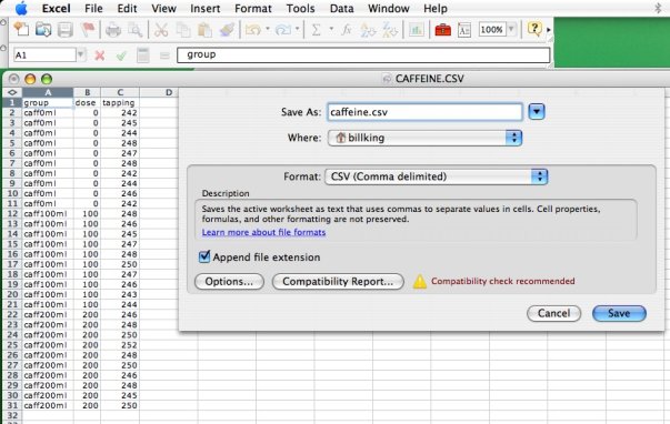

At this point, a decision must be made, which is in what form to save the file. I recommend you save it as an Excel spreadsheet first, but R will not easily read it in that form. (It's possible, but not recommended.) So you will also need to save it in plain text form, and the choices are tab separated data values, or comma separated data values.

Each form has its advantages and disadvantages. All things considered and long story short, I prefer the comma separated form, or .csv file. So after you save a copy as an Excel spreadsheet (or whatever program you are using), then save a copy as a .csv file. This is a plain text file that can be examined and modified in a text editor, and which R can read with no problem. (Excel will nag the crap out of you for trying to save as .csv, but just tell it to mind it's own business. You're not going to lose any formatting because you don't have any formatting.)

IMPORTANT NOTE: If there are commas inside of any of your data fields, in a character variable like an address, for example, the csv format will have a problem with this. On the other hand, if there are spaces in any of your data fields, the tab or whitespace separated data format might choke on that. Be careful when you're preparing your data file. Don't use commas, and don't use spaces. R can be made to work around both of these problems, but it's just easier to avoid the problem in the first place!

It wouldn't hurt you to create this file yourself, but you can also download it from this link.

caffeine.csv

Download it and save it in (or move it to) your working directory. Now to get it loaded into R, we use the read.csv() function.

> help(read.csv)

Usage
read.table(file, header = FALSE, sep = "", quote = "\"'",
           dec = ".", row.names, col.names,
           as.is = !stringsAsFactors,
           na.strings = "NA", colClasses = NA, nrows = -1,
           skip = 0, check.names = TRUE, fill = !blank.lines.skip,
           strip.white = FALSE, blank.lines.skip = TRUE,
           comment.char = "#",
           allowEscapes = FALSE, flush = FALSE,
           stringsAsFactors = default.stringsAsFactors(),
           encoding = "unknown")

read.csv(file, header = TRUE, sep = ",", quote="\"", dec=".",
         fill = TRUE, comment.char="", ...)

> caff = read.csv(file = "caffeine.csv")

> file = "http://ww2.coastal.edu/kingw/statistics/R-tutorials/text/caffeine.csv"
> caff = read.csv(file = file)         # read.csv(file) will work

Okay, so you've worked with the data frame, have done some analyses, and have made some modifications to it. Now you want to write the file back to your working directory as a .csv file that is human readable (as opposed to saving in binary format using save() as we did in a previous section, which is also possible). The function is write.csv().

> write.csv(caff, file="caffeine2.csv", row.names=FALSE)

You can also use the save() function to save the "caff" object, but the saved file will not be human readable, and it will not be readable by programs like Excel. Files saved with write.csv() can be read by any program that will read .csv files, including most statistical software (like SPSS) and virtually all spreadsheet programs and text editors.

Saving and Printing the R Console and Graphics Device

The methods for doing this are specific to different operating systems, so pick yours below. So you'll have a graphic to work with, do this.

> with(faithful, plot(waiting, eruptions))

Windows

To save a console session: 1) Click in the R Console window to bring it to focus, 2) Pull down the File menu and choose Save to File..., 3) Proceed as you would when saving any other file.

To print a console session: 1) Click in the R Console window to bring it to focus, 2) Pull down the File menu and choose Print..., 3) Be warned that this prints the entire console session, which can be VERY long. If you want to print just a part of it, highlight that part first, then follow steps 1 and 2.

To save a graphic: 1) Click in the Graphics Device window to bring it to focus, 2) Pull down the File menu, choose Save as..., and choose the desired format, 3) Proceed as you would when saving any other file. (Note: If you want to share this graphic with friends who may not be using Windows, DON'T save it as a Metadata file.)

To print a graphic: 1) Click in the Graphics Device window to bring it to focus, 2) Pull down the File menu and choose Print...

Linux

To save or print a console session: There is probably a way to do this, but I have never seen it documented. I highlight what I want to save or print, copy and paste it into a text editor like gedit, and then use that app to save or print.

To save a graphic: In an R terminal session, issue the following command...

> dev.print(file="faithful.pdf")

To print a graphic: Proceed as if you were saving (above) but leave out the file name and "file=" option. See ?dev.print for all the details.

Mac OS X

To save a console session: 1) Click in the R Console window to bring it to focus, 2) Pull down the File menu and choose Save As..., 3) Proceed as you would when saving any other file.

To print a console session: 1) Click in the R Console window to bring it to focus, 2) Pull down the File menu and choose Print..., 3) Be warned that this prints the entire console session, which can be VERY long. I don't know that there is a way, from within R, to print just a part of it. I highlight what I want, copy and paste it to a text editor, and go from there.

To save a graphic: 1) Click in the Quartz device window to bring it to focus, 2) Pull down the File menu and choose Save As..., 3) There aren't many options! The file will be saved in pdf format.

To print a graphic: 1) Click in the Quartz device window to bring it to focus, 2) Pull down the File menu and choose Print..., 3) You can also print the image to a pdf file this way.

All Operating Systems

When I say "text editor" in the above notes, I mean text editor, not word processor. If you are copying and pasting from R to a word processor, change the font in the word processor to something like courier new, or some other monospaced (typewriter-like) font. This will keep your tables and so forth aligned properly.