R Tutorials--Higher Order Repeated Measures

HIGHER ORDER ANOVA WITH REPEATED MEASURES

If you're unfamiliar with repeated measures analysis, I suggest you look at the Single Factor tutorial first.

Two Way Designs With Repeated Measures on Both Factors

We will use a data set from the MASS package called "Rabbit". The description on the help page reads as follows:

     "Five rabbits were studied on two occasions, after treatment with saline
     (control) and after treatment with the 5-HT_3 antagonist MDL 72222. After
     each treatment ascending doses of phenylbiguanide were injected intravenously
     at 10 minute intervals and the responses of mean blood pressure measured.
     The goal was to test whether the cardiogenic chemoreflex elicited by
     phenylbiguanide depends on the activation of 5-HT_3 receptors." [Note:
     5-HT_3 is a serotonin receptor.]

We will treat Treatment and Dose as factors (throwing out valuable numerical information--tsk) and, thus, we have a 2x6 factorial design with repeated measures on both factors. The response is BPchange. The subject ID is Animal.

> data(Rabbit, package="MASS")
> summary(Rabbit)
    BPchange          Dose             Run       Treatment  Animal 
 Min.   : 0.50   Min.   :  6.25   C1     : 6   Control:30   R1:12  
 1st Qu.: 1.65   1st Qu.: 12.50   C2     : 6   MDL    :30   R2:12  
 Median : 4.75   Median : 37.50   C3     : 6                R3:12  
 Mean   :11.22   Mean   : 65.62   C4     : 6                R4:12  
 3rd Qu.:20.50   3rd Qu.:100.00   C5     : 6                R5:12  
 Max.   :37.00   Max.   :200.00   M1     : 6                       
                                  (Other):24                       
> Rabbit$Dose = factor(Rabbit$Dose)              # make sure R sees your factors as factors
> with(Rabbit, table(Treatment, Dose))           # check for balance
         Dose
Treatment 6.25 12.5 25 50 100 200
  Control    5    5  5  5   5   5
  MDL        5    5  5  5   5   5
> ### a more thorough check would be table(Subject,Treatment,Dose) showing
> ### that each rabbit appears once in each of the treatment cells
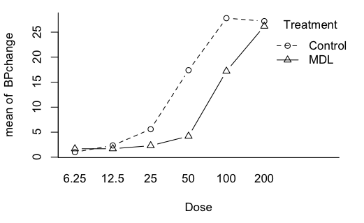
> with(Rabbit, tapply(BPchange, list(Treatment,Dose), mean))
        6.25 12.5  25   50  100  200
Control 1.00 2.35 5.6 17.4 27.8 27.2
MDL     1.68 1.69 2.3  4.2 17.2 26.2
> with(Rabbit, tapply(BPchange, list(Treatment,Dose), var))
           6.25  12.5   25   50  100  200
Control 0.15625 1.925 7.30 29.8 51.7 38.7
MDL     0.62325 0.538 1.45  8.7 62.2 47.7

We have some pretty ugly problems with the variances, but we're going to have to ignore that, as data sets for balanced ANOVA problems are few and far between in these built-in data sets. Let's see what effects we might have.

> with(Rabbit, interaction.plot(Dose,       # factor displayed on x-axis
                                Treatment,  # factor displayed as multiple lines
                                BPchange,   # the response variable
                                type="b",   # plot both points and lines
                                pch=1:2,    # use point characters 1 and 2
                                bty="l"))   # draw a box around the plot that looks like an L

As with the single factor case, the trick in doing the ANOVA is to specify a correct Error term. We want an Error term that specifies which effects are seen within subjects, and in this case that is all of them: the main effect of Dose, the main effect of Treatment, and the Dose-by-Treatment interaction. We can specify that in the Error term as follows.

> aov.out = aov(BPchange ~ Dose * Treatment + Error(Animal/(Dose*Treatment)), data=Rabbit)
> ### (Dose*Treatment) is the same as (Dose+Treatment+Dose:Treatment)
> summary(aov.out)

Error: Animal
          Df Sum Sq Mean Sq F value Pr(>F)
Residuals  4  351.4   87.86               

Error: Animal:Dose
          Df Sum Sq Mean Sq F value   Pr(>F)    
Dose       5   6022  1204.3   66.17 9.48e-12 ***
Residuals 20    364    18.2                     
---
Signif. codes:  0 '***' 0.001 '**' 0.01 '*' 0.05 '.' 0.1 ' ' 1

Error: Animal:Treatment
          Df Sum Sq Mean Sq F value Pr(>F)  
Treatment  1  328.5   328.5   13.65 0.0209 *
Residuals  4   96.3    24.1                 
---
Signif. codes:  0 '***' 0.001 '**' 0.01 '*' 0.05 '.' 0.1 ' ' 1

Error: Animal:Dose:Treatment
               Df Sum Sq Mean Sq F value   Pr(>F)    
Dose:Treatment  5  419.9   83.99   8.773 0.000156 ***
Residuals      20  191.5    9.57                     
---
Signif. codes:  0 '***' 0.001 '**' 0.01 '*' 0.05 '.' 0.1 ' ' 1

There is a significant main effect of dose. No surprise there! There is a significant main effect of Treatment, which is what we were supposedly looking for. But the main effects are complicated by the presence of a significant interaction.

Check the ANOVA table to make sure the error terms are right. Each treatment should have the corresponding subject x treatment interaction as its error term. The interaction of the treatments should have the subject x treatment x treatment interaction as its error term. Looks like we got that right! It's also a good idea to do a quick check of the degrees of freedom to make sure they are correct. One reason they might be wrong is if we failed to declare a variable coded numerically as a factor when we wanted to use it as such. Looks like we're good here, though.

The extension to the three factor completely repeated measures design is straightforward. The error term would be Error(subject/(IV1*IV2*IV3)). Be sure you use the parentheses around the names of the IVs in the "denominator" of the error term. Otherwise, your Error will be in error.

Two Way Mixed Factorial Designs

We have to be careful with the term "mixed" when we're talking about experimental designs. It is used in two very different ways: mixed factorial design and mixed model. A mixed factorial design is one that has both between and within subjects factors. A mixed model is one that has both fixed and random effects.

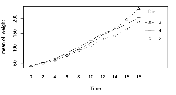
Here again we discover that the R people are not really ANOVA people. We're going to have to make do by modifying a data set that is not ideally suited to the problem. There is a data set called ChickWeight that I am going to modify to make it a balanced mixed factorial. Follow these instructions very carefully!

> data(ChickWeight)
> CW = subset(ChickWeight, as.numeric(Diet) > 1 & Time < 20)  ###  look at summaries
> CW$Diet = factor(CW$Diet, exclude="1")                        ## to see what we
> CW$Time = factor(CW$Time)                                   ###  are doing here
> summary(CW)
     weight           Time         Chick     Diet   
 Min.   : 39.0   0      : 30   24     : 10   2:100  
 1st Qu.: 62.0   2      : 30   30     : 10   3:100  
 Median :103.0   4      : 30   22     : 10   4:100  
 Mean   :113.6   6      : 30   23     : 10          
 3rd Qu.:153.2   8      : 30   27     : 10          
 Max.   :332.0   10     : 30   28     : 10          
                 (Other):120   (Other):240
> with(CW, table(Diet, Time))               # check for balance
    Time
Diet  0  2  4  6  8 10 12 14 16 18
   2 10 10 10 10 10 10 10 10 10 10
   3 10 10 10 10 10 10 10 10 10 10
   4 10 10 10 10 10 10 10 10 10 10

I believe that does it. Now we have a 3x10 mixed factorial design with repeated measures on Time (in days). There are 10 scores in each of the design cells, and those scores are the weights (in grams) of chicks on three different diets (unspecified) as it changes over time. (Note: The help page says there are 4 diets. We threw out the first one to create a balanced data set.)

> with(CW, interaction.plot(Time, Diet, weight, type="b", pch=1:3))

Once again, the secret is in getting the Error term correct. Our subject ID is Chick (and notice it is already declared a factor), and the effect that is "inside" of Chick is Time.

> aov.out = aov(weight ~ Diet * Time + Error(Chick/Time), data=CW)
> summary(aov.out)

Error: Chick
          Df Sum Sq Mean Sq F value Pr(>F)
Diet       2  10946    5473   1.562  0.228
Residuals 27  94613    3504               

Error: Chick:Time
           Df Sum Sq Mean Sq F value Pr(>F)    
Time        9 883951   98217 245.987 <2e-16 ***
Diet:Time  18  13236     735   1.842 0.0215 *  
Residuals 243  97024     399                   
---
Signif. codes:  0 '***' 0.001 '**' 0.01 '*' 0.05 '.' 0.1 ' ' 1

The correct error term for the between subjects factor is just subject variability, as usual. The correct error term for the within subjects factor is that factor crossed with subject. Same is true for the interaction. We are two for two!

Well, not so fast! Let's think about this one for a minute. What problem do you think we might have here? I'd bet my paycheck that the weight of chicks is a whole lot less variable when they are 0 days old than it is when they are 18 days old. I anticipate a serious problem with homogeneity of variance, or rather the lack thereof.

> with(CW, interaction.plot(Time,Diet,weight,fun=var,type="b",pch=1:3))   # not shown

Yikes! In the interaction.plot() function, the option fun= specifies the function you want calculated and plotted. The default is "mean", but here we used "var" to get variances. That's one of the worst problems with heterogeneity of variance I've ever seen! The largest variance is about 4000 times the smallest variance.

Three Way Designs With Repeated Measures on One Factor

We will use a built-in data set called CO2, which contains data from an experiment on the cold tolerance of the grass species Echinochloa crus-galli.

> data(CO2)
> summary(CO2)
     Plant             Type         Treatment       conc          uptake     
 Qn1    : 7   Quebec     :42   nonchilled:42   Min.   :  95   Min.   : 7.70  
 Qn2    : 7   Mississippi:42   chilled   :42   1st Qu.: 175   1st Qu.:17.90  
 Qn3    : 7                                    Median : 350   Median :28.30  
 Qc1    : 7                                    Mean   : 435   Mean   :27.21  
 Qc3    : 7                                    3rd Qu.: 675   3rd Qu.:37.12  
 Qc2    : 7                                    Max.   :1000   Max.   :45.50  
 (Other):42

"Plant" is the subject identifier. "Type" gives the geographical origin of the plant. "Treatment" tells whether the plant was chilled or not. Both of those factors are between subjects. The numeric variable "conc" is ambient carbon dioxide concentration. These values are repeated for each plant, and once again we are going to toss out valuable numerical information and make this a factor. The response is "uptake", giving carbon dioxide uptake rates.

> CO2$conc = factor(CO2$conc)
> with(CO2, table(Treatment, conc, Type))       # checking for balance
, , Type = Quebec

            conc
Treatment    95 175 250 350 500 675 1000
  nonchilled  3   3   3   3   3   3    3
  chilled     3   3   3   3   3   3    3

, , Type = Mississippi

            conc
Treatment    95 175 250 350 500 675 1000
  nonchilled  3   3   3   3   3   3    3
  chilled     3   3   3   3   3   3    3

> with(CO2, table(Plant, conc))                  # really making sure!
     conc
Plant 95 175 250 350 500 675 1000
  Qn1  1   1   1   1   1   1    1
  Qn2  1   1   1   1   1   1    1
  Qn3  1   1   1   1   1   1    1
  Qc1  1   1   1   1   1   1    1
  Qc3  1   1   1   1   1   1    1
  Qc2  1   1   1   1   1   1    1
  Mn3  1   1   1   1   1   1    1
  Mn2  1   1   1   1   1   1    1
  Mn1  1   1   1   1   1   1    1
  Mc2  1   1   1   1   1   1    1
  Mc3  1   1   1   1   1   1    1
  Mc1  1   1   1   1   1   1    1
  
> par(mfrow=c(1,2))
> with(CO2[1:42,], interaction.plot(conc, Treatment, uptake, type="b", pch=1:2, bty="l"))
> title(main="Quebec")
> with(CO2[43:84,], interaction.plot(conc, Treatment, uptake, type="b", pch=1:2, bty="l"))
> title(main="Mississippi")

Looks like those warm climate plants don't handle being chilled as well as the cold climate plants do. The error term must recognize that "conc" is the only within subjects factor. (What's wrong with these graphs? Look at the y-axes.)

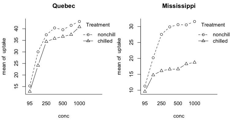
> aov.out = aov(uptake ~ Type * Treatment * conc + Error(Plant/conc), data=CO2)
> summary(aov.out)

Error: Plant
               Df Sum Sq Mean Sq F value   Pr(>F)    
Type            1   3366    3366  95.195 1.02e-05 ***
Treatment       1    988     988  27.949  0.00074 ***
Type:Treatment  1    226     226   6.385  0.03543 *  
Residuals       8    283      35                     
---
Signif. codes:  0 '***' 0.001 '**' 0.01 '*' 0.05 '.' 0.1 ' ' 1

Error: Plant:conc
                    Df Sum Sq Mean Sq F value   Pr(>F)    
conc                 6   4069   678.1 172.562  < 2e-16 ***
Type:conc            6    374    62.4  15.880 5.98e-10 ***
Treatment:conc       6    101    16.8   4.283 0.001557 ** 
Type:Treatment:conc  6    112    18.7   4.748 0.000717 ***
Residuals           48    189     3.9                     
---
Signif. codes:  0 '***' 0.001 '**' 0.01 '*' 0.05 '.' 0.1 ' ' 1

Three Way Designs With Repeated Measures on Two Factors

We have finally crapped out on built-in data sets. So we are going to have to import one. If you have an Internet connection, you can try this, typing with excruciating care. (If you don't have an Internet connection, then how are you reading these tutorials?!)

> file = "http://ww2.coastal.edu/kingw/statistics/R-tutorials/text/react.txt"
> react = read.csv(file)

If that didn't work, first carefully check your typing. If your typing is perfect, then something went wrong with the connection, either on your end or ours. Try copying and pasting this script.

### start copying here
react = read.table(header=T, sep=",", text="
subject,lab,task,color,RT
A1,A,simple,green,358
A1,A,simple,red,329
A1,A,disjunctive,green,456
A1,A,disjunctive,red,410
A1,A,choice,green,487
A1,A,choice,red,509
A2,A,simple,green,365
A2,A,simple,red,393
A2,A,disjunctive,green,394
A2,A,disjunctive,red,378
A2,A,choice,green,406
A2,A,choice,red,474
A3,A,simple,green,337
A3,A,simple,red,388
A3,A,disjunctive,green,463
A3,A,disjunctive,red,438
A3,A,choice,green,450
A3,A,choice,red,454
A4,A,simple,green,329
A4,A,simple,red,412
A4,A,disjunctive,green,453
A4,A,disjunctive,red,365
A4,A,choice,green,526
A4,A,choice,red,425
A5,A,simple,green,314
A5,A,simple,red,299
A5,A,disjunctive,green,342
A5,A,disjunctive,red,540
A5,A,choice,green,412
A5,A,choice,red,383
A6,A,simple,green,345
A6,A,simple,red,313
A6,A,disjunctive,green,399
A6,A,disjunctive,red,350
A6,A,choice,green,389
A6,A,choice,red,454
A7,A,simple,green,297
A7,A,simple,red,285
A7,A,disjunctive,green,403
A7,A,disjunctive,red,324
A7,A,choice,green,409
A7,A,choice,red,387
A8,A,simple,green,315
A8,A,simple,red,327
A8,A,disjunctive,green,333
A8,A,disjunctive,red,352
A8,A,choice,green,434
A8,A,choice,red,414
A9,A,simple,green,309
A9,A,simple,red,344
A9,A,disjunctive,green,384
A9,A,disjunctive,red,354
A9,A,choice,green,443
A9,A,choice,red,295
B1,B,simple,green,319
B1,B,simple,red,300
B1,B,disjunctive,green,396
B1,B,disjunctive,red,370
B1,B,choice,green,315
B1,B,choice,red,346
B2,B,simple,green,336
B2,B,simple,red,299
B2,B,disjunctive,green,410
B2,B,disjunctive,red,489
B2,B,choice,green,286
B2,B,choice,red,346
B3,B,simple,green,338
B3,B,simple,red,314
B3,B,disjunctive,green,341
B3,B,disjunctive,red,366
B3,B,choice,green,399
B3,B,choice,red,403
B4,B,simple,green,311
B4,B,simple,red,338
B4,B,disjunctive,green,323
B4,B,disjunctive,red,309
B4,B,choice,green,470
B4,B,choice,red,462
B5,B,simple,green,360
B5,B,simple,red,308
B5,B,disjunctive,green,434
B5,B,disjunctive,red,386
B5,B,choice,green,395
B5,B,choice,red,375
B6,B,simple,green,314
B6,B,simple,red,311
B6,B,disjunctive,green,383
B6,B,disjunctive,red,369
B6,B,choice,green,372
B6,B,choice,red,381
B7,B,simple,green,356
B7,B,simple,red,313
B7,B,disjunctive,green,380
B7,B,disjunctive,red,354
B7,B,choice,green,339
B7,B,choice,red,356
B8,B,simple,green,325
B8,B,simple,red,320
B8,B,disjunctive,green,363
B8,B,disjunctive,red,408
B8,B,choice,green,352
B8,B,choice,red,369
B9,B,simple,green,305
B9,B,simple,red,312
B9,B,disjunctive,green,343
B9,B,disjunctive,red,344
B9,B,choice,green,377
B9,B,choice,red,373
")
### end copying here and paste into the R Console

> summary(react)
    subject   lab             task      color          RT       
 A1     : 6   A:54   choice     :36   green:54   Min.   :285.0  
 A2     : 6   B:54   disjunctive:36   red  :54   1st Qu.:328.5  
 A3     : 6          simple     :36              Median :365.0  
 A4     : 6                                      Mean   :372.3  
 A5     : 6                                      3rd Qu.:403.8  
 A6     : 6                                      Max.   :540.0  
 (Other):72

Both of these methods worked for me. Hopefully, one worked for you. These data were collected in an undergraduate experimental psychology lab. There were two lab sections ("lab"), A and B, with 9 students in each section, so this is a between subjects factor. Each student did three different kinds of reaction time task ("task"), simple, disjunctive, and choice, so this is a within subjects factor. In addition, each student did each task with two different colors of stimulus lights ("color"), green and red, so this is also a within subjects variable. The response was reaction time in milliseconds. So we have a 2x3x2 factorial design with repeated measures on factors two and three.

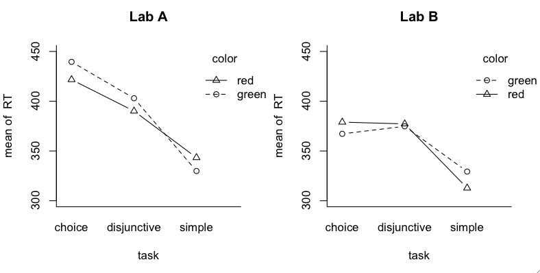
The experiment was similar to studies done by Donders in the 19th century in which he was attempting to measure the amount of time it takes a mental event to occur (mental chronometry it was called). Simple reaction time tasks are quite simple. You see a stimulus, and you react to it as quickly as you possibly can. Disjunctive tasks are a little more complex, in that two (or more, but two here) different stimuli might be presented, and you are only to respond to one of them. So in addition to the time it takes to react, there is also a decision to make: should I react or not. Finally, in choice reaction time tasks, there are two (or more) different stimuli, and each requires a different response. So the decision has become more complex: which response should I make.

> with(react, tapply(RT, list(color, task, lab), mean))    # means
, , A

        choice disjunctive   simple
green 439.5556    403.0000 329.8889
red   421.6667    390.1111 343.3333

, , B

        choice disjunctive   simple
green 367.2222    374.7778 329.3333
red   379.0000    377.2222 312.7778

> with(react, tapply(RT, list(color, task, lab), var))     # variances
, , A

        choice disjunctive    simple
green 1906.278    2248.500  536.8611
red   3908.500    4333.611 1992.2500

, , B

        choice disjunctive   simple
green 2851.944    1282.944 382.5000
red   1291.000    2507.694 133.6944

The largest variance is 4333.6/133.7=32.4 times as large as the smallest one, once again problematic, and once again something we try to pretend isn't a problem. (I don't advocate this, but just to get an example of this design under our belts, we'll look the other way.

> condition = paste(react$lab, react$task, react$color,sep=".")
> bartlett.test(react$RT ~ condition)

	Bartlett test of homogeneity of variances

data:  react$RT by condition
Bartlett's K-squared = 31.7706, df = 11, p-value = 0.0008301

Ouch! Let's hurry on.

> par(mfrow=c(1,2))
> with(react[1:54,], interaction.plot(task, color, RT, 
+      type="b", pch=1:2, bty="l", ylim=c(300,450)))
> title(main="Lab A")
> with(react[55:108,], interaction.plot(task, color, RT,
+      type="b", pch=1:2, bty="l", ylim=c(300,450)))       # y-axis same on both graphs
> title(main="Lab B")

I'm not sure why R does that little trick with the legends (reversing the order of the levels), but I can live with it. If I need it not to be that way, I can draw a custom legend. Let's move on to the ANOVA. Both task and color as well as their interaction are within subjects, so...

> aov.out = aov(RT ~ lab * task * color + Error(subject/(task*color)), data=react)
> summary(aov.out)

Error: subject
          Df Sum Sq Mean Sq F value  Pr(>F)   
lab        1  26289   26289   8.756 0.00923 **
Residuals 16  48039    3002                   
---
Signif. codes:  0 '***' 0.001 '**' 0.01 '*' 0.05 '.' 0.1 ' ' 1

Error: subject:task
          Df Sum Sq Mean Sq F value   Pr(>F)    
task       2 106509   53255  23.591 5.06e-07 ***
lab:task   2   9448    4724   2.093     0.14    
Residuals 32  72238    2257                     
---
Signif. codes:  0 '***' 0.001 '**' 0.01 '*' 0.05 '.' 0.1 ' ' 1

Error: subject:color
          Df Sum Sq Mean Sq F value Pr(>F)
color      1    290   290.1   0.260  0.617
lab:color  1    169   168.7   0.151  0.702
Residuals 16  17831  1114.4               

Error: subject:task:color
               Df Sum Sq Mean Sq F value Pr(>F)
task:color      2     61    30.6   0.020  0.980
lab:task:color  2   4366  2182.8   1.428  0.255
Residuals      32  48899  1528.1

There are two significant main effects, lab and task. Task I expected. Lab I have no explanation for considering the very simple nature of the response.

A Final Note

I don't know how to do these problems in R using a multivariate approach. If anyone does, please clue me in.

created 2016 February 9