R Tutorials--Probability Distributions

PROBILITY DISTRIBUTIONS, QUANTILES, CHECKS FOR NORMALITY

Probability Distributions

R has density and distribution functions built-in for about 20 probability distributions, including those in the following table.

distribution	function	type
binomial	binom	discrete
chi-squared	chisq	continuous
F	f	continuous
hypergeometric	hyper	discrete
normal	norm	continuous
Poisson	pois	discrete
Student's t	t	continuous
uniform	unif	continuous

By prefixing a "d" to the function name in the table above, you can get probability density values (pdf). By prefixing a "p", you can get cumulative probabilities (cdf). By prefixing a "q", you can get quantile values. By prefixing an "r", you can get random numbers from the distribution. I will demonstrate using the normal distribution.

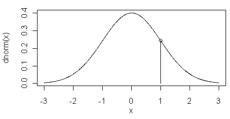
The dnorm() function returns the height of the normal curve at some value along the x-axis. This is illustrated in the figure at left. Here the value of dnorm(1) is shown by the vertical line at x=1.

> dnorm(1)         # d for density
[1] 0.2419707

With no options specified, the value of "x" is treated as a standard score or z-score. To change this, you can specify "mean=" and "sd=" options. In other words, dnorm() returns the probability density function or pdf.

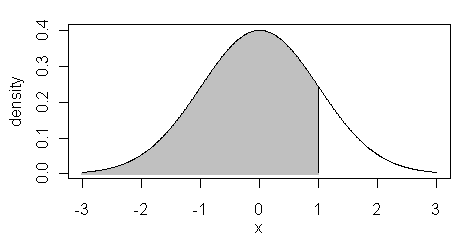
The pnorm() function is the cumulative density function or cdf. It returns the area below the given value of "x", or for x=1, the shaded region in the figure at right.

> pnorm(1)
[1] 0.8413447

Once again, the defaults for mean and sd are 0 and 1 respectively. These can be set to other values as in the case of dnorm(). To find the area above the cutoff x-value, either subtract from 1, or set the "lower.tail=" option to FALSE.

> 1 - pnorm(1)          # think of it as a p-value, which makes the p in pnorm easier to remember
[1] 0.1586553
> pnorm(1, lower.tail=F)
[1] 0.1586553

So, good news! No more tables!

To get quantiles or "critical values", you can use the qnorm() function as in the following examples.

> qnorm(.95)                           # p = .05, one-tailed (upper)
[1] 1.644854
> qnorm(c(.025,.975))                  # p = .05, two-tailed
[1] -1.959964  1.959964
> qnorm(seq(from=.1,to=.9,by=.1))      # deciles from the unit normal dist.
[1] -1.2815516 -0.8416212 -0.5244005 -0.2533471  0.0000000  0.2533471  0.5244005
[8]  0.8416212  1.2815516

Once again, there are "mean=" and "sd=" options.

To use these functions with other distributions, more parameters may need to be given. Here are some examples.

> pt(2.101, df=8)                      # area below t = 2.101, df = 8
[1] 0.9655848
> qchisq(.95, df=1)                    # critical value of chi square, df = 1
[1] 3.841459
> qf(c(.025,.975), df1=3, df2=12)      # quantiles from the F distribution
[1] 0.06975178 4.47418481
> dbinom(60, size=100, prob=.5)        # a discrete binomial probability
[1] 0.01084387

The help pages for these functions will give the necessary details.

Random numbers are generated from a given distribution like this.

> runif(9)                             # 9 uniformly distributed random nos.
[1] 0.01961714 0.62086249 0.64193142 0.99583719 0.06294405 0.94324289 0.88233387
[8] 0.11851026 0.60300929
> rnorm(9)                             # 9 normally distributed random nos.
[1] -0.95186711  0.09650050 -0.37148202  0.56453509 -0.44124876 -0.43263580
[7] -0.46909466  1.38590806 -0.06632486
> rt(9, df=10)                         # 9 t-distributed random nos.
[1] -1.538466123 -0.249067184 -0.324245905 -0.009964799  0.143282490
[6]  0.619253016  0.247399305  0.691629869 -0.177196453

One again, I refer you to the help pages for all the gory details.

Empirical Quantiles

Suppose you want quartiles or deciles or percentiles or whatever from a sample or empirical distribution. The appropriate function is quantile(). From the help page for this function, the syntax is...

quantile(x, probs = seq(0, 1, 0.25), na.rm = FALSE,
         names = TRUE, type = 7, ...)

This says "enter a vector, x, of data values, or the name of such a vector, and I will return quantiles for positions 0, .25, .5, .75, and 1 (in other words, quartiles along with the min and max values), without removing missing values (and if missing values exist the function will fail and return an error message), I'll give each of the returned values a name, and I will use method 7 (of 9) to do the calculations." Let's see this happen using the built-in data set "rivers".

> quantile(rivers)
  0%  25%  50%  75% 100% 
 135  310  425  680 3710

Compare this to what you get with a summary.

> summary(rivers)
   Min. 1st Qu.  Median    Mean 3rd Qu.    Max. 
  135.0   310.0   425.0   591.2   680.0  3710.0

So what's the point? The quantile() function is much more versatile because you can change the default "probs=" values.

> quantile(rivers, probs=seq(.2,.8,.2))     # quintiles
20% 40% 60% 80% 
291 375 505 735 
> quantile(rivers, probs=seq(.1,.9,.1))     # deciles
 10%  20%  30%  40%  50%  60%  70%  80%  90% 
 255  291  330  375  425  505  610  735 1054 
> quantile(rivers, probs=.55)               # 55th percentile
55% 
460
> quantile(rivers, probs=c(.05,.95))        # and so on
  5%  95% 
 230 1450

And then there is the "type=" option. It turns out there is some disagreement among different sources as to just how quantiles should be calculated from an empirical distribution. R doesn't take sides. It gives you nine different methods! Pick the one you like best by setting the "type=" option to a number between 1 and 9. Here are some details (and more are available on the help page): type=2 will give the results most people are taught to calculate in an intro stats course, type=3 is the SAS definition, type=6 is the Minitab and SPSS definition, type=7 is the default and the S definition and seems to work well when the variable is continuous.

Checks For Normality

Parametric procedures like the t-test, F-test (ANOVA), and Pearson r assume the data are distributed normally, or are sampled from a normally distributed population, to be more precisely correct. There are several ways to check this assumption.

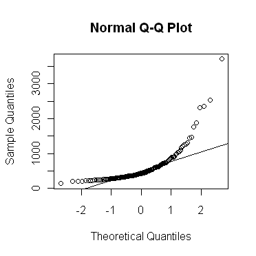
The qqnorm() function allows a graphical evaluation.

> qqnorm(rivers)

If the values in the vector are close to normally distributed, the points on the plot will fall (more or less) along a straight line. This line can be plotted on the graph like this.

> qqline(rivers)

As you can see, the "rivers" vector is strongly skewed, as indicated by the bowing of the points up away from the expected straight line. The very long upper tail (strong positive skew) in this distribution could also have been visualized using...

> plot(density(rivers))

...the output of which is not shown here. You can see this in the QQ plot as well by the fact that the higher sample values are much too large to be from a theoretical normal distribution. The lower tail of the distribution appears to be a bit short.

Statistical tests for normality are also available. Perhaps the best known of these is the Shapiro-Wilk test.

> shapiro.test(rivers)

        Shapiro-Wilk normality test

data:  rivers 
W = 0.6666, p-value < 2.2e-16

I believe we can safely reject the null hypothesis of normality here! Here's a question for all you stat students out there: how often should the following result in a rejection of the null hypothesis if our random number generator is worth its salt?

> shapiro.test(rnorm(100))

        Shapiro-Wilk normality test

data:  rnorm(100) 
W = 0.9894, p-value = 0.6192

This question will be on the exam!

Another test that can be used here is the Kolmogorov-Smirnov test.

> ks.test(rivers, "pnorm", alternative="two.sided")

        One-sample Kolmogorov-Smirnov test

data:  rivers 
D = 1, p-value < 2.2e-16
alternative hypothesis: two-sided 

Warning message:
In ks.test(rivers, "pnorm", alternative = "two.sided") :
  cannot compute correct p-values with ties

But it gets upset when there are ties in the data. Inside the function, the value "pnorm" tells the test to compare the empirical cumulative density function of "rivers" to the cumulative density function of a normal distribution. The null hypothesis says the two will match. Clearly they do not, so the null hypothesis is rejected. We conclude once again, and for the last time in this tutorial, that "rivers" is not normally distributed.

Most statisticians seem to be of the opinion that the graphical methods are the better way of evaluating normality when the evaluation is being done to check the normality assumption of a statistical test such as the t-test. The significance tests of normality, so I'm told, are too sensitive to violations when the sample is large and not sensitive enough when the sample is small.

revised 2016 January 26