R Tutorials by William B. King, Ph.D.
| Table of Contents | Function Reference | Function Finder | R Project |

PRELIMINARIES


A Warning

Take my word for this. Not everything will make sense to you at first! If there is anything that puzzles you, don't worry. You will probably see it illustrated in the tutorials to come. R can't be learned "all at once." It will take repeated exposures, and (YO, STUDENTS!) practice. I will not be showing you much output in this tutorial, and that is quite intentional. If you want to see it, look at your open R Console.

A special warning to my students: I've been teaching a long time, and I know how hard it is to get you to practice things. These are your tools. It's your responsibility to learn to use them, and you're not going to do that by watching me or by skimming over a tutorial. Sit down at a computer, open R, and GET TO WORK! If you're not willing to put in the time, I suggest you find some other course to take, because you're not going to pass this one! I will NOT answer questions about R during the exams.


What is R?

First, there was S. The S statistical programming language was developed in the late 1970's, primarily by John Chambers at Bell Labs. S was first distributed outside of Bell Labs in 1980, and by 1988 the "New S Language" had become available. This was the basis for the commercial version called S-Plus. By 1990, S or S-Plus was in widespread use by statisticians.

In the early 1990's, Ross Ihaka and Robert Gentleman, of the University of Auckland in New Zealand, wrote a teaching version of S/S-Plus and named it R. In 1995 the source code for R was released as open source under the Gnu Public License. People who are unfamiliar with this concept are encouraged to click those links and read all about it. Since that time, R has become one of the most powerful and versatile statistical software programs available at any price.

R is a statistical computing environment. Primarily, it is a programming language, but one containing a very large number of statistical functions. These functions can be used to perform complex statistical analyses interactively, or they can be included in larger scripts and programs to accomplish even more complex tasks. R also has very elaborate graphical capabilities, allowing the production of publication-quality graphics.

R is free software. To get R, simply go to the R Project homepage and download it. Click on the CRAN link on the lefthand side of the page under downloads. (CRAN stands for Comprehensive R Archive Network.) R is available for Windows (Windows 95 and later), Mac OS X, and Linux. As of this writing (15 January 2016), the latest version is 3.2.3. A new version is released about once or twice a year.

Once you have R, you may do almost anything with it you please. You can install it on as many computers as you want. You can examine and modify the source code. You can even resell it, as long as you make the source code available. Unlike commerical software such as SPSS, you are not paying an exorbitant fee to "rent" a restricted-use copy. R is free!


The R Prompt

Start R like you would start any other program on your computer. In Windows, the R installer will place a shortcut icon on your desktop. On the Mac, you will have to drag an icon from your Applications folder to the dock. In Linux, R runs from a terminal window. You can also run R from either terminal.app or an X11 terminal on a Mac. I wouldn't recommend this in Windows, however.

R is command-line driven. This means you type your commands at a prompt rather than hunting and clicking through menus. This is much faster and more versatile than a GUI (graphical user interface), but it does take some getting used to for those of you who rarely take your hands off your mouse or get a kick from smearing your fingerprints all over your screen.

R GUIs are in development. Google up "R Commander" for example. The S-Plus commercial version also has a GUI, but be ready to pay dearly for it, in cash money, that is. (Note: S-Plus was at one time sold by Insightful, which is now owned by TIBCO and appears to have been rebranded as Spotfire S+.)

For those of you who haven't seen it previously in the install help or work-along demo tut, this is what R will look like (more or less--this is the Mac verison) when it opens. This window is called the R Console. (In Windows, it will have a larger gray window behind it. This is normal.)

R Console

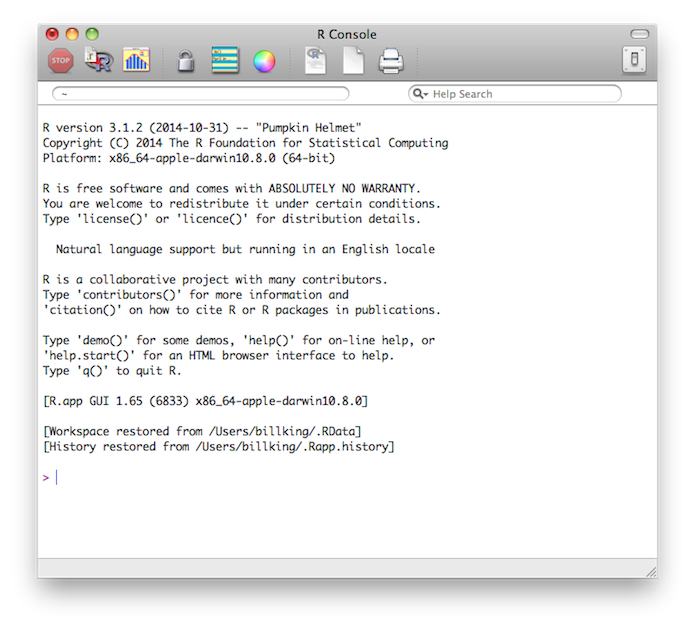
The R prompt is the greater than symbol, >, at the bottom of that window. When you see it, start typing. If your command is a long one and breaks onto the next line, or if you hit Enter without completing a command, R will prompt you on the next line with a plus sign (+). This means "you ain't done yet--gimme more." This often happens when you don't close a parenthesis. For example...

> oneway.test(weight ~ group, data = PlantGrowth      # Note: press Enter here
+                                                     # Type ) and press Enter here
You neglected to close the open left parenthesis. Close it and hit Enter and everything will be fine. R is not too picky about how you type your commands as far as spacing is concerned, but it will insist that parentheses (and quotes) come in left and right pairs. By the way, go ahead and type the commands that you see here into R. The data objects required to make these examples work are built in to R for educational purposes. Just remember that R is case sensitive, so in addition to parentheses, you will also have to get capitalization (and spelling) correct.

Notes: In the newer versions of R on the Mac, parentheses (and quotes) are closed for you. I.e., as soon as you type the left one, the right one also appears. This can be very convenient; in some cases, it can also be annoying. A common trick that programmers use is to type left and right parentheses at the same time, then backspace with the arrow keys and type whatever goes between them.

Further note: In some versions of R, especially those on Windows, when your typing reaches the right side of the window, R does not break the line but scrolls the window to the right. Once again, convenient and annoying. You can insert a break yourself by hitting the Enter key, if you prefer the window not to jump around. The Mac command editor will automatically break the line when it hits the right side of the editor window.

Final note: Sometimes you will get stuck at the + prompt. That's probably because you made a syntax error before the line broke, and now it can't be fixed by just typing more at the command prompt. You will have to abort the command and start over. This is done by pressing the Escape (Esc) key in the upper left corner of the keyboard. MAKE A NOTE OF THIS. You're going to need to know it eventually.


Quitting R

Best to know this right away, I suppose. To quit R, type...

> quit()
...and then press the Enter (or Return) key. You always tell R to execute a command line by pressing the Enter key. By the way, q() is a shortcut for "quit" and will also work.

The parentheses are mandatory, even though there is nothing inside them. R will ask if you wish to save your workspace. Say yes if you want to save any of the objects (data) you created while working in R. (See the next tutorial for "objects.")


Case Sensitive

R is case sensitive. "My_data" and "my_data" are not the same objects. Nor are Anova() and anova() the same functions (commands). The most common reason I get error messages is capitalizing where I shouldn't have, or not where I should have. If you get an "unknown object" or "function not found" error, check your capitalization first. And then check your spelling! The vast majority of R commands are all lower case (and must be typed that way!), but there are exceptions.

This might also be a good place to point out that R does not like spaces in the names of things. Use a dot or an underline character instead. Thus, "my.data" and "my_data" are fine (and different) names for a data set, but "my data" is not allowed. "MyData" and "myData" are also allowed (and different) names for data objects. But don't use a dash: "my-data". R will think you mean subtraction: "my" minus "data". You should follow these rules not only for named data objects you create while using R, but also in files you save with R. I.e., don't put spaces in filenames. R will usually work around it if you do, but it's just better to avoid the potential hassle to begin with.


Comment Lines

R code, like any good programming code, can be commented. Any line or partial line in R beginning with the hash or pound symbol (#) is a comment, or note, and R will ignore it. You can use these to annotate your analysis or make notes to yourself (or others). Type the following. Remember to press the Enter key at the end of each line.

> # This is just a note.
> ### And so is this.
> summary(rivers)                      # And so is this.
> # In the last command line, R will summarize the "rivers" variable and 
> # ignore all these notes. Try it and see!
If you are going to save your R session (explained in a future tutorial), liberal comments will help you remember what you've done. (STUDENTS: When you see comments in my handouts, you do not need to type that part!)


R Functions

Almost every command you issue in R will take the form of a function. Functions have the following syntax.

> function.name(arguments, options)
For example...
> mean(islands, na.rm = T)
This function takes the mean of a variable called "islands", the argument. The option, na.rm=T, tells R to remove missing values, if any, before doing so. R will not calculate the mean of a variable that has missing values unless you tell it that the missing values should be removed. Unlike some statistical software, R is clever enough to know that variables with missing values don't have means.

The parentheses are manditory, even if there are no arguments or options given. For example...

> ls()
If you type the name of a function without the parentheses, R will show you how the function is coded; i.e., it will print out the programming code for the function. I mention this because it can be startling to the unwary! It's harmless though. You haven't broken anything. Try it! Type ls and leave off the parentheses. By the way, you can scroll the R console window with your mouse to see the stuff that scrolled off the screen. Don't expect it to make much sense to you though.


A Taste--Before You Get Too Impatient!

If you haven't already, fire up R and get to typing. I'll illustrate a few more interesting and important features of R in these examples.

For educational purposes, R has a large number of data sets built into it. I will use these to illustrate a few things R can do. When you start R, you will get a screen something like this. This is the aforementioned R Console. It will be in it's own window on Mac and Windows. In Linux, R runs in the terminal.

     R version 2.10.1 (2009-12-14)
     Copyright (C) 2009 The R Foundation for Statistical Computing
     ISBN 3-900051-07-0

     R is free software and comes with ABSOLUTELY NO WARRANTY.
     You are welcome to redistribute it under certain conditions.
     Type 'license()' or 'licence()' for distribution details.

       Natural language support but running in an English locale

     R is a collaborative project with many contributors.
     Type 'contributors()' for more information and
     'citation()' on how to cite R or R packages in publications.

     Type 'demo()' for some demos, 'help()' for on-line help, or
     'help.start()' for an HTML browser interface to help.
     Type 'q()' to quit R.

     [Previously saved workspace restored]

     >

The R core team and R developers the world over are volunteers doing this, well, maybe not entirely out of the goodness of their hearts, but without much compensation. They would like you to cite them if you use R for data analysis. To see how to do this, issue the following command.

> citation()
Congratulations! You're an R user! (And a special note to my STUDENTS using this tutorial: You are REQUIRED to cite R if you use it for your data analysis or graphics.)

To give you a bit of an idea of what R is capable of graphically, try this.

> demo("graphics")
You will get a message telling you to "Type <Return> to start". This means press the Enter (or Return) key. When you do, a gray graphics window will open and some stuff will print out in the R Console window. You can ignore how these things are coded (for now). Just watch the graphics window. In the R Console it says "Waiting to confirm page change..." This means press Enter again. If nothing happens, be sure the R Console window has focus (i.e., click in the R Console window somewhere), and then press Enter again. Each time you press Enter, a new graph will appear. There are about 11 in all. R's graphics capabilities are pretty impressive, and this is just a small sample. When you are done admiring the graphs (when the graphs stop changing upon hitting Enter), close the graphics window like you would any other window on your system.

This little exercise has placed a lot of stuff in your workspace (to be explained later). We should clean that up. WARNING: The command I am about to tell you to execute will erase everything in your workspace, and that will be permanent. If you've been using R already, and there is something in your workspace you want to save, save it now!

> ls()                  # List the contents of the workspace.
> rm(list=ls())         # This completely clears the workspace. There is also a menu item for this.
> ls()
character(0)            # This means "nothing to see here."
In Windows and on the Mac, you can also manage your workspace via menus. In Windows, use your mouse to put down the "Misc" menu and choose "List objects" to see the contents of your workspace. (It seems to me that typing ls() is a lot easier!) Pull down "Misc" and choose "Remove all objects" to clear the workspace. On the Mac, you use the "Workspace" menu to accomplish the same things. Choose "Show workspace" and "Clear workspace" to do so. Now let's look at some data.

As a brief appetite whetting, let's look at a data set called "HairEyeColor". This is a table showing a crosstabulation of hair color, eye color, and sex (gender) for 592 statistics students. Type this, and don't type the command prompt--R has already supplied that for you. Remember to press Enter to execute the command.

> data(HairEyeColor)         # Put the data in your workspace.
> HareEyeColor               # An intentional error. Get used to seeing this message!
Error: object 'HareEyeColor' not found
> HairEyeColor               # Remember to watch your capitalization! And spelling!
Since "HairEyeColor" is already a defined object (more on this later), typing its name will cause R to display it. This is actually a shortcut for the function...
> print(HairEyeColor)
...which does the same thing, but allows some options to be applied. You should now be looking at a three-dimensional (4x4x2) crosstabulation in your R console. The following command will show you the names of the variables as well as the levels of them.
> dimnames(HairEyeColor)
Here is another way you can visualize this information, called a flat table.
> ftable(HairEyeColor)
> ftable(HairEyeColor, col.vars="Eye")
> ftable(HairEyeColor, row.vars=c("Sex","Hair"), col.vars="Eye")
Don't like typing a data name that long? Make a copy with a shorter name, which you can use below any place you see the full name.
> HEC = HairEyeColor
> ftable(HEC)
A chi-square test for independence of all factors in the table (log linear analsysis) can be done as follows.
> summary(HairEyeColor)                # or summary(HEC)
Number of cases in table: 592 
Number of factors: 3 
Test for independence of all factors:
        Chisq = 164.92, df = 24, p-value = 5.321e-23
        Chi-squared approximation may be incorrect
> 
Because the p-value is so small, R has printed it in scientific notation: 5.321x10⁻²³. You need to know this notation to use R. Whenever you see a number followed immediately by a lower case "e" and then another number, that "e" part means "times ten to this exponent". If the exponent is positive, this is a very large number; if negative, a very small number (i.e., very close to zero). If you are unfamiliar with or don't remember scientific notation for large and small numbers, you will need to learn it. Click this link for a brief lesson: Scientific Notation. (STUDENTS: You cannot report this number as 5.321. That's not partial credit. That's just wrong! Okay, a compromise. I'll give you 1e-23 points for it.)

The null hypothesis that all factors are independent (i.e., no interactions between any factors) is rejected. If you are getting error messages instead of statistical output, remember: R is case sensitive. HairEyeColor and haireyecolor and NOT the same thing. (Note: The warning message "Chi-squared approximation may be incorrect" means there are expected frequencies less than 5.)

You are not to worry about the details of this syntax at this point. This is just for show! To collapse over one or more of the factors in this table, you can do one of these.

> margin.table(HairEyeColor, c(1,2))     # collapses over sex (i.e., displays vars 1 & 2)
> margin.table(HairEyeColor, c(2,3))     # collapses over hair color
> margin.table(HairEyeColor, c(1,3))     # collapses over eye color
> margin.table(HairEyeColor, c(1))       # collapses over eye color and sex
Curiously, this will not work. They should really fix this!
> margin.table(HEC, c("Hair","Eye"))
Error in margin.table(HEC, c("Hair", "Eye")) : 
  the dims contain missing values
But if we really want it to work, we can make it work.
> Hair=1;Eye=2;Sex=3                   # Multiple commands same line separated by semicolons.
> margin.table(HEC, c(Hair,Eye))       # When to quote and when not to quote--takes getting used to!
Suppose we wanted to see that first margin table again, but didn't want to go scrolling around for it, and didn't want to retype the command. R remembers everything you've typed at the command prompt. Just hit the up-arrow key to recall previous commands one at a time. When you get back to the command you want to execute again (or edit and execute), press Enter. Up-arrow, up-arrow, up-arrow, up-arrow, up-arrow, up-arrow, up-arrow, Enter does it for me.

Suppose we wished to perform an ordinary (i.e., two-way) Pearson chi-square test of independence on hair color and eye color just for the men. Here's how to do it (and once again, just for show so don't worry about memorizing all this syntax, which probably won't make much sense to you at this point).

> chisq.test(HairEyeColor[,,1])        # All levels of Hair, all levels of Eye, first level of Sex.

        Pearson's Chi-squared test

data:  HairEyeColor[, , 1] 
X-squared = 41.2803, df = 9, p-value = 4.447e-06

Warning message:
In chisq.test(HairEyeColor[, , 1]) :
  Chi-squared approximation may be incorrect
The test indicates a relationship between hair color and eye color. However, there is a warning that the result may not be accurate. This warning occurs when the expected frequencies may not be high enough to make the chi square approximation accurate. In this case there is one cell of the 16 with an expected value less than 5, and it has EF=4, so I wouldn't worry too much about it. To see these expected values, type...
> chisq.test(HairEyeColor[,,1])$expected
       Eye
Hair       Brown     Blue     Hazel     Green
  Black 19.67025 20.27240  9.433692  6.623656
  Brown 50.22939 51.76703 24.089606 16.913978
  Red   11.94265 12.30824  5.727599  4.021505
  Blond 16.15771 16.65233  7.749104  5.440860
Warning message:
In chisq.test(HairEyeColor[, , 1]) :
  Chi-squared approximation may be incorrect

R is nothing if not flexible. To see the data in yet another format, try this.
> as.data.frame.table(HairEyeColor)
Want to see proportions instead of raw frequencies?
> prop.table(HairEyeColor[,,1], margin=1)   # relative to row marginal sums
> prop.table(HairEyeColor[,,1], margin=2)   # relative to column marginal sums
Okay, I think we've whetted ourselves enough for now. There are a few more details we need to cover before we can get down to some data analysis.


Some Definitions

workspace
The workspace is the area of your computer's memory (RAM) where R is storing the variables and other things you are currently working with. To see the contents of the workspace...

> ls()
[1] "HairEyeColor" "HEC"
The ls() function stands for "list the objects in my workspace". An equivalent function is...
> objects()
Your output may be different if you've been fooling around with R or not cleaning out your workspace after some of the above examples. If the output says character(0), this means there is nothing in your workspace because you haven't created or stored anything there. If you do this...
> x = 7
...an object called "x" is created in your workspace (and any older object named "x" is overwritten without warning, so be careful). We can see it like so.
> ls()
[1] "HairEyeColor" "HEC"          "x"
To remove an object from your workspace, use either rm() or remove().
> rm(x)
> ls()
[1] "HairEyeColor" "HEC"
> remove(HEC)
> ls()
[1] "HairEyeColor"
It's a good idea to keep your workspace clean. When you have finished using an object, remove it so it doesn't get in the way when you begin your next analysis. Be aware though that in R removing stuff from your workspace is permanent. It cannot be recovered from the trash. A future tutorial will deal with how to save a permanent copy of something.

There is one more consequence of your workspace being in RAM. If the power goes out, or your laptop battery goes dead, your workspace is gone! If you're worried about this, you can always do a quick save of your workspace as follows.

> save.image()
This saves a copy of your workspace to the working directory in a file called ".RData". It accomplishes exactly the same thing as saying "yes" when R asks you if you want to save your workspace at shutdown.

working directory
This is a directory (or "folder" for those of you who have been spoiled by Windows) on your hard drive or other storage device where R will look when you ask it to read in a file. It is also where R will try to save something if you ask to save a file. To find out what's in your working directory, type this. Not all of it will be R stuff unless you've created a folder just for R (a good idea).

> dir()
 [1] "Jordan_Data.xls"        "BandK.csv"             
 [3] "R_functions"            "Rspace_071025"         
 [5] "Rspace_test"            "Sex2.csv"              
 [7] "Smith Logic file.xls"   "UCB.saved"             
 [9] "age_chd.txt"            "coronary.csv"          
[11] "data_folder"            "death_penalty"         
[13] "elephants.txt"          "elephants_analysis.odt"
[15] "elevCA_smoke_chd.txt"   "eysenck.csv"           
[17] "garafola_mullet"        "hack_altered.csv"      
[19] "hack_altered.sav"       "hackett_data.csv"      
[21] "logic_file.csv"         "police_log.saved"      
[23] "testdir"               
>
First, take a moment to notice how R numbers things it prints to the console (screen). In this output there are 23 objects (files), and each of them has a number. Only the first one on each line of output is numbered, however. This number appears in square brackets at the beginning of the line. So "Jordan_Data.xls" is the first item in this output, "BandK.csv" is the second, "R_functions" is the third, and so on. Remember this. It will be important later.

You can identify your working directory as follows.

> getwd()                         # get pathname to my working directory
[1] "/Users/billking/Rspace"
It's a good idea, in my opinion, not to use your home directory (in Windows XP it's My Documents, in Vista and I suspect Windows 7 it's your home folder, on the Mac and in Linux it's your home folder) as the R working directory. So, as you can see in the above example, I have created a directory called "Rspace" inside the home directory (inside My Documents on my WinXP computer, and inside billking on my Mac) to use with R. I changed to it, and then viewed its contents, like this (don't type these commands just yet).
> setwd("Rspace")
> dir()
IMPORTANT NOTE to everyone: In the tutorials that follow, I will assume you are in a working directory called Rspace. So create that working directory now. There is a way to do that from within R, but it doesn't always work, so just use your operating system to do it. Go to Finder (Mac) or Windows Explorer (or whatever they're calling it on Windows these days), click your way to whatever getwd( ) has identified as your working directory, and create a new folder there called Rspace (right click - New folder...). Then when you start R, use setwd( ) to change to that directory (i.e., make it your working directory). You can also set the working directory from a menu item if you care to hunt around for it (Misc > Change Working Directory... on a Mac). And there is also a profile file you can modify to do this automatically upon startup, but I suspect if you understand that, you can figure it out, and if you don't, I probably shouldn't bother you with it! (The file is called .Rprofile and should be created in your default working directory.)
> setwd("Rspace")
> getwd()
[1] "/Users/billking/Rspace"
From here on, at the beginning of every tutorial, you should begin by executing the command setwd("Rspace"), provided you haven't created a .Rprofile file with that command in it.

search path
When you ask R to do a calculation on an object, R will look in the search path to find that object. It will also look in the search path to find the function you are asking to execute. If it fails to find either one, you'll get an error message like "object not found" or "function not found". To see your search path...

> search()
[1] ".GlobalEnv"        "package:stats"     "package:graphics" 
[4] "package:grDevices" "package:utils"     "package:datasets" 
[7] "package:methods"   "Autoloads"         "package:base"
>
This is the Windows result, but it will be similar in any other OS. The first entry is your "global environment," also called your workspace. This is the first place R will look for anything you ask it to use. The rest are various tools and packages. We will find out how to add places to your search path in future tutorials.

Lot's of stuff to remember, right? Don't worry too much about it right now. Working with something is the best way to learn it. If you use it, the knowledge will come! (Okay, apologies to W. P. Kinsella for that one!)


Getting Help

To see a manual page in R for any function, type...
> help("function.name")           # a shortcut is ?function.name
For example...
> help("mean")                    # or just ?mean
I should point out that these help screens will open in separate windows on the Mac and in Windows. These windows can be manipulated with the mouse just like any other window on your screen. When you're done looking at, click the appropriate button to close it. In Linux, the help screens appear in-line with your R session in the R Console. To get back to your command prompt, press q (lower case Q).

These manual pages are intended for experts and can seem inpenetrable until you learn a little more about R. Don't worry about them for now. However, if you're daring and want to see a worked example, try this.

> example("mean")
(In my opinion, many of the worked examples this and many other functions produce are unnecessarily complex. They are definitely not intended for beginners, that's for sure!)

If you don't know the name of the function you want, there is a way around that. For example, suppose you want to calculate a median but don't know the function to do so. Try this.

> help.search("median")
This will give you a list of functions, all of which have something to do with the median. From looking through this list, you should be able to spot the median() function. Most R commands are this cryptic!

If you are looking for a function that does a "mean-like sort of thing", and you're not quite sure what it's called, but you're pretty sure that "mean" is part of its name, do this.

> apropos("mean")
The output will be every R function (in the search path) that has "mean" as part of its name.

There are also R manuals online (and they also come with the download, so you have them already on your hard drive). The two most important ones are "An Introduction to R," and "R Data Import/Export." They can be found here:

http://www.cran.r-project.org/manuals.html

By the way, CRAN stands for Comprehensive R Archive Network. There are many tons of useful stuff online there.


A Final Preliminary Word or Two

Don't expect to understand R all at once! This is a full-featured statistical programming language and analysis environment. You will never understand it all. R will do everything from 2+2 to factor analysis and generalized linear (and nonlinear) models. If you need it done, R will probably do it. I recently had to use a relatively new technique called generalized estimating equations. There weren't at that time many software packages out there that will do it, but R will. I had to download an optional package from the CRAN site, but that's easy enough to do.

If there is something in these tutorials that puzzles you, make a note of it and move on. Ask someone when you have a chance, or wait for it to come up again in a later tutorial. Perhaps it will be explained more fully there. Or try the help (manual) page, but don't pin your hopes on those just yet. Reading those is a skill in itself. It took me quite awhile to get used to them. Try googling it. That usually works for me.


A Final Final Word

Most of the data sets used in the tutorials that follow are either built in to R, i.e., you get them with the download, or are available at this website. See the About The Data Sets document for details.


revised 2016 January 15
| Table of Contents | Function Reference | Function Finder | R Project |