
MULTIPLE REGRESSION WITH INTERACTIONS Preliminary Notes "Seriously? This has to be covered separately?" I'm afraid it does. Interaction of continuous variables is not a simple thing. Some people refer to the analysis of interactions in multiple regression as moderator analysis and to the interacting variable as a moderating variable. I'll talk a little about that below, but moderator analysis is only a subset of interaction analysis. I'll be discussing one particular type of interaction, called a bilinear interaction, which is represented in the regression equation as a product term. You should be aware that there are other ways that continuous variables can interact. Failing to find a significiant product term in a multiple regression analysis is not sufficient evidence to say that the variables are not interacting. Also, if you haven't read the Model Formulae tutorial yet, well, I'm sure by now you know the drill. It would also be helpful if you were familiar with Multiple Regression. (Come on, King! Did you really need to say that?) Product Terms and What They Mean In the case of simple linear regression, our analysis resulted in a regression equation of this form. Y-hat = b0 + b1X Y-hat stands for the predicted value of Y and is usually written as a Y with a caret symbol, ^, over it. I'm not sure I can program that it HTML, and even if I could, there's no guarantee that your browser would faithfully reproduce it. The traditional reading of the symbol is "Y hat". I don't want to type that a whole lot, but I also don't want to simply use Y because students, especially, often forget that we are using the regression equation to calculate predicted values of Y, and not the actual observed values. So I'm going to break with precedent and use Pr to stand for the predicted value we get from a regression equation. And since I'm not a big fan of subscripts, especially when I have to program them into HTML, that will allow me to use X, Y, and Z as the predictor variables in place of X1, etc. So our simple linear regression equation becomes... Pr = b0 + b1X In multiple regression without interactions, we added more predictors to the regression equation. Pr = b0 + b1X + b2Y Pr = b0 + b1X + b2Y + b3Z Etc. In principle, there is no limit to the number of predictors that can be added, although with n subjects, once we get to k-1 predictors, no matter what they are, we are making perfect predictions and learning nothing. So generally we are advised to hold it down to a reasonable, i.e., parsimonious, number of predictors. To test for the presence of an interaction between X and Y, customarily an XY product term is added to the equation. Pr = b0 + b1X + b2Y + b3XY As I've already pointed out, that's not the only way that predictors can interact, but when you ask your software to test for an interaction, that's almost certainly the test you're going to get, unless you go to some trouble to specify something different. That will be the test you get in R if you use the X:Y or X*Y notation in the model formula. What does it mean? In the case of simple linear regression (one predictor), the regression equation specifies the graph of a straight line, called the regression line. In the case of multiple regression with two predictors and no interaction, the regression line become a regression plane in 3D space. (Don't try to visualize what it is with more predictors. You could sprain your visual cortex!) 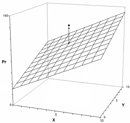
The plane represents the predicted values (Pr), but the actual or observed values, in most cases, will not be on the plane but some distance above or below it. The vertical distance from a predicted value to the corresponding observed value is called a residual. Points above the plane, like the illustrated one, have positive residuals. Points below the plane have negative residuals. All of the lines in the grid representing this plane are straight. (Geometrically, they are "lines," not "curves.") All of the lines running from left to right have the same slope, which is the value of b1 in the regression equation, and is called the effect of X (sometimes the main effect of X). All of the lines running from front to back have the same slope, which is the value of b2 in the regression equation, and is called the effect of Y (sometimes the main effect of Y). The point where the plane touches the Pr axis is the intercept, which has the value b0 in the regression equation. Add a product interaction term, b3XY, and this causes the plane to become twisted. Not bowed, twisted. All of the lines in the grid are still straight (they are still "lines"), but the lines running from left to right no longer all have the same slope, and the lines running from front to back no longer all have the same slope. 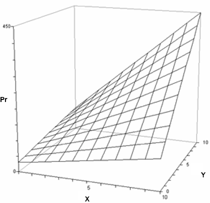
Each of the lines in this grid running from left to right (and all other lines that you might imagine doing so) are called simple effects of X. Likewise, all of the lines running from front to back are called simple effects of Y. Those simple effects are still linear, hence, bilinear interaction. But notice that the size of any simple effect of X depends upon the value of Y, and the size of any simple effect of Y depends upon the value of X. This can be shown from the regression equation with a little bit of algebra. Pr = b0 + b1X + b2Y + b3XY The slope of any line going from left to right, a simple effect of X, is b1 + b3Y. The slope of any line going from front to back, a simple effect of Y, is b2 + b3X. Thus, the coefficient of the product term, b3, specifies how much the simple effect of X changes as Y changes, and how much the simple effect of Y changes as X changes. Perhaps most importantly, without the product term (interaction), b1 is the effect of X at any value of Y, and b2 is the effect of Y at any value of X. Hence, the coefficients are rightfully referred to as "effects." With an interaction in force, that is no longer true. With a product term, b1 now represents the effect of X only when Y is equal to 0, and b2 represents the effect of Y only when X is equal to 0. In other words, b1 and b2 are now simple effect of X and Y when the other equals 0. You might want to study the above diagram for a moment to get the full implications of this. Notice that X can have a pretty big effect on Pr, but when Y=0, the effect of X is minimal. Same for Y. Finally, An Example! I'm going to try to figure out what variables are related to gas mileage in
cars using some data from the 1970s (because that's the kinda guy I am). The
built-in data set is called "mtcars", and I'm going to take only some of the
variables available in it to keep things "simple."
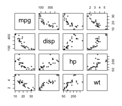
Let's check to see if the relationships are reasonably linear.
In the last tutorial, we got additive models by separating the predictors
in the model formula with plus signs. Now we want models including the
interactions, so instead of using +, we use asterisks, *.
The first thing we have to remember is that, other than the three-way interaction, we're not looking at effects. Our regression equation is of this form. Pr = b0 + b1X + b2Y + b3Z + b4XY + b5XZ + b6YZ + b7XYZ Therefore, just to look at one example...Pr = b0 + (b1 + b4Y + b5Z + b7YZ)X + b2Y + b3Z + b6YZ We're not looking at "an effect of X." We're looking at a simple effect of X (displacement) when Y (horsepower) and Z (weight) are both 0. We should know immediately, that's not interesting! How many cars do you think there were back in the 1970s with zero horsepower and zero weight? I'm guessing, not a lot! (Today maybe, but not in the seventies.)Something else that should have clued us in here is that, even though we have no significant coefficients (no coefficients significantly different from zero), we have R2 = .89, which is "off the charts" significant, F(7,24) = 27.82, p = 5x10⁻¹⁰. There's something useful in there somewhere! If you have the "car" package installed (see
Package Management), you can do this to see another problem we're having.
No matter how many problems we fix, however, that three-way interaction is
never going to get any better, so I suggest we drop it and proceed from there.
Let's fix the "meaningless simple effects" problem by making 0 a meaningful
value for each of the predictors. We do that by a procedure called mean
centering. To do that, we transform each of the variables by subtracting
the mean, creating a mean-centered variable. That will make 0 the mean of
each of those variables, and that will make the simple effects shown in the
regression output, for example, the simple effect of X at the
means of Y and Z (because the means now happen to be 0 if we use the
centered version of these variables).
However, notice that the evaluation of the interactions hasn't changed at
all. Should we just toss them out and go with an additive model? Let's not get
impatient! Let's compare the additive model to the one we currently have.
Model Reduction We now have three choices, so far as I can see. We can use theory (something we know about cars) to pick one of those interactions to delete. Or we could start by deleting the least significant one. Or we could use a stepwise regression to delete terms. In any event, once we start our process of model simplification, we should do it ONE TERM AT A TIME. Anybody know enough about cars to pick one of those interactions to delete?
Not me. I'm going to run the stepwise regression, but I'm not going to look at
the result until I've pruned this model by hand. Then I'll check to see if the
computer agrees with me.
Of the three variables we started with, we have retained horsepower and weight
and their mutual interaction. Let's see how we're doing with variance inflation.
> confint(lm.out, level=.99)
                 0.5 %       99.5 %
(Intercept) 17.5286437 20.268156481
hp.c        -0.0512404 -0.009774873
wt.c        -5.5949569 -2.668341231
hp.c:wt.c    0.0073459  0.048350396
What Does The Interaction Look Like? There are several plots that can be used to visualize interactions, but I
prefer the conditioning plot. It has a lot of options. I'll try to illustrate
the most important ones.
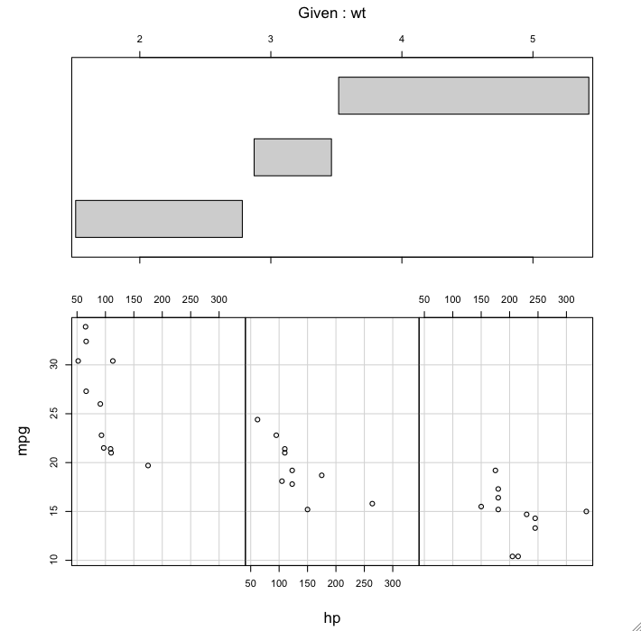
The top panel shows the ranges of "wt" that are covered in each of the graphs. The bottom panel shows a scatterplot of "mpg" by "hp" within each of those ranges. The only other option I might have set here was "panel=panel.smooth", which would have plotted a smoothed regression line on each of the plots. And possibly "show.given=F", which would turn off the top panel of the graphic. You can play with the options to see how they alter the graph. The only necessary parts are the formula and the data= argument. The coplot is telling us that, at low values of vehicle weight, the relationship between mpg and hp is very steep. That is, gas mileage drops off rapidly as horsepower increases. At moderate values of vehicle weight the relationship is less steep but still strongly negative. Finally, at high vehicle weights, increasing horsepower has much less effect but still appears to be slightly negative. Moderator Effects In many cases, our primary interest is in one of our predictors, which we think has a causal relationship to the response. The causal relationship must be justified through the way we designed the experiment, randomization to groups for example, or through some theoretical consideration. Let's say our primary interest in this example is in the predictor variable engine horsepower (hp). However, we don't think the relationship between gas mileage and horsepower is a simple, straightforward one. Rather, we think the precise form of the relationship depends upon the weight of the vehicle. In other words, we think weight is a moderator variable. If it is, then the moderator effect will show up as a horsepower-by-weight interaction in the regression analysis. Fred, in the lab across the street, is primarily interested in the relationship between gas mileage and the weight of the vehicle. He thinks the precise form of that relationship is altered depending upon the horsepower of the engine. Thus, to Fred, horsepower is the moderator variable. The key element of moderator analysis is our belief that the influences we are seeing are causal. We can't say, in many regression analyses, what kind of causal relationship there might be between our variables. If we are trying to predict college GPA from SAT scores, for example, we can't really say that SAT scores cause GPA. There is clearly a relationship that we can use for prediction and decision making, but it's not a causal one. Therefore, if we include a variable that we think interacts with SAT in our analysis, we shouldn't really call what we're doing a moderator analysis. Not all interactions are moderator effects. Furthermore, in a moderator effect, unlike in a mediator effect, neither
the IV nor the moderator variable have causal priority. They don't act
directly on each other. They both act simultaneously, more or less, through the
dependent variable. Finally, "it is desirable that the moderator variable be
uncorrelated with both the predictor and the criterion (the dependent variable)
to provide a clearly interpretable interaction term" (Baron and Kenny, 1986).
created 2016 March 27 |