R Tutorials--Logistic Regression

LOGISTIC REGRESSION

Preliminaries

Model Formulae

You will need to know a bit about Model Formulae to understand this tutorial.

Odds, Odds Ratios, and Logit

When you go to the track, how do you know which horse to bet on? You look at the odds. In the program, you may see the odds for your horse, Sea Brisket, are 8 to 1, which are the odds AGAINST winning. This means in nine races Sea Brisket would be expected to win 1 and lose 8. In probability terms, Sea Brisket has a probability of winning of 1/9, or 0.111. But the odds of winning are 1:8, 1/8, or 0.125. Odds are actually the ratio of two probabilities.

                         p(one outcome)       p(success)    p
               odds = -------------------- = ----------- = ---, where q = 1 - p
                      p(the other outcome)    p(failure)    q

So for Sea Brisket, odds(winning) = (1/9)/(8/9) = 1/8. Notice that odds have these properties:

If p(success) = p(failure), then odds(success) = 1 (or 1 to 1, or 1:1).
If p(success) < p(failure), then odds(success) < 1.
If p(success) > p(failure), then odds(success) > 1.
Unlike probability, which cannot exceed 1, there is no upper bound on odds.

The natural log of odds is called the logit, or logit transformation, of p: logit(p) = log_e(p/q). Logit is sometimes called "log odds." Because of the properties of odds given in the list above, the logit has these properties:

If odds(success) = 1, then logit(p) = 0.
If odds(success) < 1, then logit(p) < 0.
If odds(success) > 1, then logit(p) > 0.
The logit transform fails if p = 0.

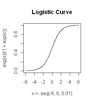
Logistic regression is a method for fitting a regression curve, y = f(x), when y consists of proportions or probabilities, or binary coded (0,1--failure, success) data. When the response is a binary (dichotomous) variable, and x is numeric, logistic regression fits a logistic curve to the relationship between x and y. The logistic curve looks like the graph at right. It is an S-shaped or sigmoid curve, often used to model population growth, survival from a disease, the spread of a disease (or something disease-like, such as a rumor), and so on. The logistic function is...

y = [exp(b₀ + b₁x)] / [1 + exp(b₀ + b₁x)]

Logistic regression fits b₀ and b₁, the regression coefficients (which were 0 and 1, respectively, for the graph above). It should have already struck you that this curve is not linear. However, the point of the logit transform is to make it linear.

logit(y) = b₀ + b₁x

Hence, logistic regression is linear regression on the logit transform of y, where y is the proportion (or probability) of success at each value of x. However, you should avoid the temptation to do a traditional least-squares regression at this point, as neither the normality nor the homoscedasticity assumption will be met.

The odds ratio might best be illustrated by returning to our horse race. Suppose in the same race, Seattle Stew is given odds of 2 to 1 against, which is to say, two expected loses for each expected win. Seattle Stew's odds of winning are 1/2, or 0.5. How much better is this than the winning odds for Sea Brisket? The odds ratio tells us: 0.5 / 0.125 = 4.0. The odds of Seattle Stew winning are four times the odds of Sea Brisket winning. Be careful not to say "times as likely to win," which would not be correct. The probability (likelihood, chance) of Seattle Stew winning is 1/3 and for Sea Brisket is 1/9, resulting in a likelihood ratio of 3.0. Seattle Stew is three times more likely to win than is Sea Brisket.

Logistic Regression: One Numeric Predictor

In the "MASS" library there is a data set called "menarche" (Milicer, H. and Szczotka, F., 1966, Age at Menarche in Warsaw girls in 1965, Human Biology, 38, 199-203), in which there are three variables: "Age" (average age of age homogeneous groups of girls), "Total" (number of girls in each group), and "Menarche" (number of girls in the group who have reached menarche). Menarche Graph

> library("MASS")
> data(menarche)
> str(menarche)
'data.frame':   25 obs. of  3 variables:
 $ Age     : num   9.21 10.21 10.58 10.83 11.08 ...
 $ Total   : num  376 200 93 120 90 88 105 111 100 93 ...
 $ Menarche: num  0 0 0 2 2 5 10 17 16 29 ...
> summary(menarche)
      Age            Total           Menarche      
 Min.   : 9.21   Min.   :  88.0   Min.   :   0.00  
 1st Qu.:11.58   1st Qu.:  98.0   1st Qu.:  10.00  
 Median :13.08   Median : 105.0   Median :  51.00  
 Mean   :13.10   Mean   : 156.7   Mean   :  92.32  
 3rd Qu.:14.58   3rd Qu.: 117.0   3rd Qu.:  92.00  
 Max.   :17.58   Max.   :1049.0   Max.   :1049.00
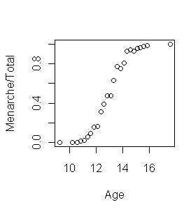
> plot(Menarche/Total ~ Age, data=menarche)

From the graph at right, it appears a logistic fit is called for here. The fit would be done this way.

> glm.out = glm(cbind(Menarche, Total-Menarche) ~ Age, family=binomial(logit), data=menarche)

Numerous explanation are in order! First, glm() is the function used to do generalized linear models. With "family=" set to "binomial" with a "logit" link, glm() produces a logistic regression. Because we are using glm() with binomial errors in the response variable, the ordinary assumptions of least squares linear regression (normality and homoscedasticity) don't apply. Second, our data frame does not contain a row for every case (i.e., every girl upon whom data were collected). Therefore, we do not have a binary (0,1) coded response variable. No problem! If we feed glm() a table (or matrix) in which the first column is number of successes and the second column is number of failures, R will take care of the coding for us. In the above analysis, we made that table on the fly inside the model formula by binding "Menarche" and "Total − Menarche" into the columns of a table (matrix) using cbind().

Let's look at how closely the fitted values from our logistic regression match the observed values.

> plot(Menarche/Total ~ Age, data=menarche)
> lines(menarche$Age, glm.out$fitted, type="l", col="red")
> title(main="Menarche Data with Fitted Logistic Regression Line")

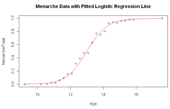I'm impressed! The numerical results are extracted like this.

> summary(glm.out)

Call:
glm(formula = cbind(Menarche, Total - Menarche) ~ Age, family = binomial(logit), 
    data = menarche)

Deviance Residuals: 
    Min       1Q   Median       3Q      Max  
-2.0363  -0.9953  -0.4900   0.7780   1.3675  

Coefficients:
             Estimate Std. Error z value Pr(>|z|)    
(Intercept) -21.22639    0.77068  -27.54   <2e-16 ***
Age           1.63197    0.05895   27.68   <2e-16 ***
---
Signif. codes:  0 '***' 0.001 '**' 0.01 '*' 0.05 '.' 0.1 ' ' 1 

(Dispersion parameter for binomial family taken to be 1)

    Null deviance: 3693.884  on 24  degrees of freedom
Residual deviance:   26.703  on 23  degrees of freedom
AIC: 114.76

Number of Fisher Scoring iterations: 4

The following requests also produce useful results: glm.out$coef, glm.out$fitted, glm.out$resid, glm.out$effects, and anova(glm.out).

Recall that the response variable is log odds, so the coefficient of "Age" can be interpreted as "for every one year increase in age the odds of having reached menarche increase by exp(1.632) = 5.11 times."

To evaluate the overall performance of the model, look at the null deviance and residual deviance near the bottom of the print out. Null deviance shows how well the response is predicted by a model with nothing but an intercept (grand mean). This is essentially a chi square value on 24 degrees of freedom, and indicates very little fit (a highly significant difference between fitted values and observed values). Adding in our predictors--just "Age" in this case--decreased the deviance by 3667 points on 1 degree of freedom. Again, this is interpreted as a chi square value and indicates a highly significant decrease in deviance. The residual deviance is 26.7 on 23 degrees of freedom. We use this to test the overall fit of the model by once again treating this as a chi square value. A chi square of 26.7 on 23 degrees of freedom yields a p-value of 0.269. The null hypothesis (i.e., the model) is not rejected. The fitted values are not significantly different from the observed values.

Logistic Regression: Multiple Numerical Predictors

During the Fall semester of 2005, two students in our program--Rachel Mullet and Lauren Garafola--did a senior research project in which they studied a phenomenon called Inattentional Blindness (IB). IB refers to situations in which a person fails to see an obvious stimulus right in front of his eyes. (For details see this website.) In their study, Rachel and Lauren had subjects view an online video showing college students passing basketballs to each other, and the task was to count the number of times students in white shirts passed the basketball. During the video, a person in a black gorilla suit walked though the picture in a very obvious way. At the end of the video, subjects were asked if they saw the gorilla. Most did not!

Rachel and Lauren hypothesized that IB could be predicted from performance on the Stroop Color Word test. This test produces three scores: "W" (word alone, i.e., a score derived from reading a list of color words such as red, green, black), "C" (color alone, in which a score is derived from naming the color in which a series of Xs are printed), and "CW" (the Stroop task, in which a score is derived from the subject's attempt to name the color in which a color word is printed when the word and the color do not agree). The data are in the following table, in which the response, "seen", is coded as 0=no and 1=yes.

gorilla = read.table(header=T, text="
seen   W   C CW
   0 126  86 64
   0 118  76 54
   0  61  66 44
   0  69  48 32
   0  57  59 42
   0  78  64 53
   0 114  61 41
   0  81  85 47
   0  73  57 33
   0  93  50 45
   0 116  92 49
   0 156  70 45
   0  90  66 48
   0 120  73 49
   0  99  68 44
   0 113 110 47
   0 103  78 52
   0 123  61 28
   0  86  65 42
   0  99  77 51
   0 102  77 54
   0 120  74 53
   0 128 100 56
   0 100  89 56
   0  95  61 37
   0  80  55 36
   0  98  92 51
   0 111  90 52
   0 101  85 45
   0 102  78 51
   1 100  66 48
   1 112  78 55
   1  82  84 37
   1  72  63 46
   1  72  65 47
   1  89  71 49
   1 108  46 29
   1  88  70 49
   1 116  83 67
   1 100  69 39
   1  99  70 43
   1  93  63 36
   1 100  93 62
   1 110  76 56
   1 100  83 36
   1 106  71 49
   1 115 112 66
   1 120  87 54
   1  97  82 41
")

We might begin like this.

> cor(gorilla)                         # a correlation matrix
            seen           W          C         CW
seen  1.00000000 -0.03922667 0.05437115 0.06300865
W    -0.03922667  1.00000000 0.43044418 0.35943580
C     0.05437115  0.43044418 1.00000000 0.64463361
CW    0.06300865  0.35943580 0.64463361 1.00000000

Or like this.

> with(gorilla, tapply(W, seen, mean))
        0         1 
100.40000  98.89474 
> with(gorilla, tapply(C, seen, mean))
       0        1 
73.76667 75.36842 
> with(gorilla, tapply(CW, seen, mean))
       0        1 
46.70000 47.84211

The Stroop scale scores are moderately positively correlated with each other, but none of them appears to be related to the "seen" response variable, at least not to any impressive extent. There doesn't appear to be much here to look at. Let's have a go at it anyway. Since the response is a binomial variable, a logistic regression can be done as follows.

> glm.out = glm(seen ~ W * C * CW, family=binomial(logit), data=gorilla)
> summary(glm.out)

Call:
glm(formula = seen ~ W * C * CW, family = binomial(logit), data = gorilla)

Deviance Residuals: 
    Min       1Q   Median       3Q      Max  
-1.8073  -0.9897  -0.5740   1.2368   1.7362  

Coefficients:
              Estimate Std. Error z value Pr(>|z|)  
(Intercept) -1.323e+02  8.037e+01  -1.646   0.0998 .
W            1.316e+00  7.514e-01   1.751   0.0799 .
C            2.129e+00  1.215e+00   1.753   0.0797 .
CW           2.206e+00  1.659e+00   1.329   0.1837  
W:C         -2.128e-02  1.140e-02  -1.866   0.0621 .
W:CW        -2.201e-02  1.530e-02  -1.439   0.1502  
C:CW        -3.582e-02  2.413e-02  -1.485   0.1376  
W:C:CW       3.579e-04  2.225e-04   1.608   0.1078  
---
Signif. codes:  0 '***' 0.001 '**' 0.01 '*' 0.05 '.' 0.1 ' ' 1 

(Dispersion parameter for binomial family taken to be 1)

    Null deviance: 65.438  on 48  degrees of freedom
Residual deviance: 57.281  on 41  degrees of freedom
AIC: 73.281

Number of Fisher Scoring iterations: 5

> anova(glm.out, test="Chisq")
Analysis of Deviance Table

Model: binomial, link: logit

Response: seen

Terms added sequentially (first to last)


       Df Deviance Resid. Df Resid. Dev P(>|Chi|)
NULL                      48     65.438          
W       1    0.075        47     65.362     0.784
C       1    0.310        46     65.052     0.578
CW      1    0.106        45     64.946     0.745
W:C     1    2.363        44     62.583     0.124
W:CW    1    0.568        43     62.015     0.451
C:CW    1    1.429        42     60.586     0.232
W:C:CW  1    3.305        41     57.281     0.069

Two different extractor functions have been used to see the results of our analysis. What do they mean?

The first gives us what amount to regression coefficients with standard errors and a z-test, as we saw in the single variable example above. None of the coefficients are significantly different from zero (but a few are close). The deviance was reduced by 8.157 points on 7 degrees of freedom, for a p-value of...

> 1 - pchisq(8.157, df=7)
[1] 0.3189537

Overall, the model appears to have performed poorly, showing no significant reduction in deviance (no significant difference from the null model).

The second print out shows the same overall reduction in deviance, from 65.438 to 57.281 on 7 degrees of freedom. In this print out, however, the reduction in deviance is shown for each term, added sequentially first to last. Of note is the three-way interaction term, which produced a nearly significant reduction in deviance of 3.305 on 1 degree of freedom (p = 0.069).

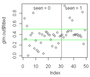
In the event you are encouraged by any of this, the following graph might be revealing.

> plot(glm.out$fitted)
> abline(v=30.5,col="red")
> abline(h=.3,col="green")
> abline(h=.5,col="green")
> text(15,.9,"seen = 0")
> text(40,.9,"seen = 1")

I'll leave it up to you to interpret this on your own time. (Also, try running the anova() tests on a model in which CW has been entered first.)

Logistic Regression: Categorical Predictors

Let's re-examine the "UCBAdmissions" data set, which we looked at in a previous tutorial.

> ftable(UCBAdmissions, col.vars="Admit")
            Admit Admitted Rejected
Gender Dept                        
Male   A               512      313
       B               353      207
       C               120      205
       D               138      279
       E                53      138
       F                22      351
Female A                89       19
       B                17        8
       C               202      391
       D               131      244
       E                94      299
       F                24      317

The data are from 1973 and show admissions by gender to the top six grad programs at the University of California, Berkeley. Looked at as a two-way table, there appears to be a bias against admitting women.

> dimnames(UCBAdmissions)
$Admit
[1] "Admitted" "Rejected"

$Gender
[1] "Male"   "Female"

$Dept
[1] "A" "B" "C" "D" "E" "F"

> margin.table(UCBAdmissions, c(2,1))
        Admit
Gender   Admitted Rejected
  Male       1198     1493
  Female      557     1278

However, there are also relationships between "Gender" and "Dept" as well as between "Dept" and "Admit", which means the above relationship may be confounded by "Dept" (or "Dept" might be a lurking variable, in the language of traditional regression analysis). Perhaps a logistic regression with the binomial variable "Admit" as the response can tease these variables apart.

If there is a way to conveniently get that flat table into a data frame (without splitting an infinitive), I don't know it. So I had to do this. (I'll leave off the command prompts so you can copy and paste it.)

### begin copying here
ucb.df = data.frame(gender=rep(c("Male","Female"),c(6,6)),
                    dept=rep(LETTERS[1:6],2),
                    yes=c(512,353,120,138,53,22,89,17,202,131,94,24),
                    no=c(313,207,205,279,138,351,19,8,391,244,299,317))
### end copying here and paste into the R Console

> ucb.df
   gender dept yes  no
1    Male    A 512 313
2    Male    B 353 207
3    Male    C 120 205
4    Male    D 138 279
5    Male    E  53 138
6    Male    F  22 351
7  Female    A  89  19
8  Female    B  17   8
9  Female    C 202 391
10 Female    D 131 244
11 Female    E  94 299
12 Female    F  24 317

Once again, we do not have a binary coded response variable, so the last two columns of this data frame will have to be bound into the columns of a table (matrix) to serve as the response in the model formula.

> mod.form = "cbind(yes,no) ~ gender * dept"     # mind the quotes here!
> glm.out = glm(mod.form, family=binomial(logit), data=ucb.df)

I used a trick here of storing the model formula in a data object, and then entering the name of this object into the glm() function. That way, if I made a mistake in the model formula (or want to run an alternative model), I have only to edit the "mod.form" object to do it.

Let's see what we have found.

> options(show.signif.stars=F)         # turn off significance stars (optional)
> anova(glm.out, test="Chisq")
Analysis of Deviance Table

Model: binomial, link: logit

Response: cbind(yes, no)

Terms added sequentially (first to last)


            Df Deviance Resid. Df  Resid. Dev   P(>|Chi|)
NULL                           11      877.06            
gender       1    93.45        10      783.61   4.167e-22
dept         5   763.40         5       20.20  9.547e-163
gender:dept  5    20.20         0  -2.265e-14   1.144e-03

This is a saturated model, meaning we have used up all our degrees of freedom, and there is no residual deviance left over at the end. Saturated models always fit the data perfectly. In this case, it appears the saturated model is required to explain the data adequately. If we leave off the interaction term, for example, we will be left with a residual deviance of 20.2 on 5 degrees of freedom, and the model will be rejected (p = .001144). It appears all three terms are making a significant contribution to the model.

How they are contributing appears if we use the other extractor.

> summary(glm.out)

Call:
glm(formula = mod.form, family = binomial(logit), data = ucb.df)

Deviance Residuals: 
 [1]  0  0  0  0  0  0  0  0  0  0  0  0

Coefficients:
                 Estimate Std. Error z value Pr(>|z|)
(Intercept)        1.5442     0.2527   6.110 9.94e-10
genderMale        -1.0521     0.2627  -4.005 6.21e-05
deptB             -0.7904     0.4977  -1.588  0.11224
deptC             -2.2046     0.2672  -8.252  < 2e-16
deptD             -2.1662     0.2750  -7.878 3.32e-15
deptE             -2.7013     0.2790  -9.682  < 2e-16
deptF             -4.1250     0.3297 -12.512  < 2e-16
genderMale:deptB   0.8321     0.5104   1.630  0.10306
genderMale:deptC   1.1770     0.2996   3.929 8.53e-05
genderMale:deptD   0.9701     0.3026   3.206  0.00135
genderMale:deptE   1.2523     0.3303   3.791  0.00015
genderMale:deptF   0.8632     0.4027   2.144  0.03206

(Dispersion parameter for binomial family taken to be 1)

    Null deviance:  8.7706e+02  on 11  degrees of freedom
Residual deviance: -2.2649e-14  on  0  degrees of freedom
AIC: 92.94

Number of Fisher Scoring iterations: 3

These are the regression coefficients for each predictor in the model, with the base level of each factor being suppressed. Remember, we are predicting log odds, so to make sense of these coefficients, they need to be "antilogged".

> exp(-1.0521)                         # antilog of the genderMale coefficient
[1] 0.3492037
> 1/exp(-1.0521)
[1] 2.863658

This shows that men were actually at a significant disadvantage when department and the interaction are controlled. The odds of a male being admitted were only 0.35 times the odds of a female being admitted. The reciprocal of this turns it on its head. All else being equal, the odds of female being admitted were 2.86 times the odds of a male being admitted. (Any excitement we may be experiencing over these "main effects" should be tempered by the fact that we have a significant interaction that needs interpreting.)

Each coefficient compares the corresponding predictor to the base level. So...

> exp(-2.2046)
[1] 0.1102946

...the odds of being admitted to department C were only about 1/9th the odds of being admitted to department A, all else being equal. If you want to compare, for example, department C to department D, do this.

> exp(-2.2046) / exp(-2.1662)          # C:A / D:A leaves C:D
[1] 0.962328

All else equal, the odds of being admitted to department C were 0.96 times the odds of being admitted to department D.

To be honest, I'm not sure I'm comfortable with the interaction in this model. It seems to me the last few calculations we've been doing would make more sense without it. You might want to examine the interaction, and if you think it doesn't merit inclusion, run the model again without it. Try doing that entering "dept" first.

> mod.form="cbind(yes,no) ~ dept + gender"
> glm.out=glm(mod.form, family=binomial(logit), data=ucb.df)
> anova(glm.out, test="Chisq")

Statistics are nice, but in the end it's what makes sense that should rule the day.

revised 2016 February 19