
| Table of Contents
| Function Reference
| Function Finder
| R Project |
INDEPENDENT SAMPLES t TEST
Syntax
The syntax for the t.test() function is given
here from the help page in R.
## Default S3 method:
t.test(x, y = NULL,
       alternative = c("two.sided", "less", "greater"),
       mu = 0, paired = FALSE, var.equal = FALSE,
       conf.level = 0.95, ...)

## S3 method for class 'formula':
t.test(formula, data, subset, na.action, ...)
"S3" refers to the S language (version 3), which is often the same as the
methods and syntax used by R. In the case of the
t.test() function, there
are two alternative syntaxes, the default, and the "formula" syntax. Both
syntaxes are relevant to the two-sample t-tests. The default syntax requires
two data vectors, "x" and "y", to be specified. To get the independent measures
t-test, leave the option "paired=" set to FALSE.
The "alternative=" option is set by default to "two.sided" but can
be set to any of the three values shown above. The default null hypothesis is
"mu = 0", which in this case should be read as "mu1-mu2=0". This is usually what
we want, but doesn't have to be, and should be changed by the user if this is
not the null hypothesis. The "var.equal=" option determines whether or not the
variances are pooled to estimate the population variance. The default is no
(FALSE). The rest can be ignored for the moment.
The t Test With Two Independent Groups
As part of his senior research project in the Fall semester of 2001, Scott
Keats looked for a possible relationship between marijuana smoking and a deficit
in performance on a task measuring short term memory--the digit span task from
the Wechsler Adult Intelligence Scale. Two groups of ten subjects were tested.
One group, the "nonsmokers," claimed not to smoke marijuana. A second group, the
"smokers," claimed to smoke marijuana regularly. The data set is small and
easily entered by hand with c() or scan(). I'll leave off the command prompts so you can copy
and paste these two lines if you want to take the easy way out. (Actually, it's
so I can do it, but I didn't want to admit it.)
nonsmokers = c(18,22,21,17,20,17,23,20,22,21)
smokers = c(16,20,14,21,20,18,13,15,17,21)
The values of the response variable indicate number of items completed
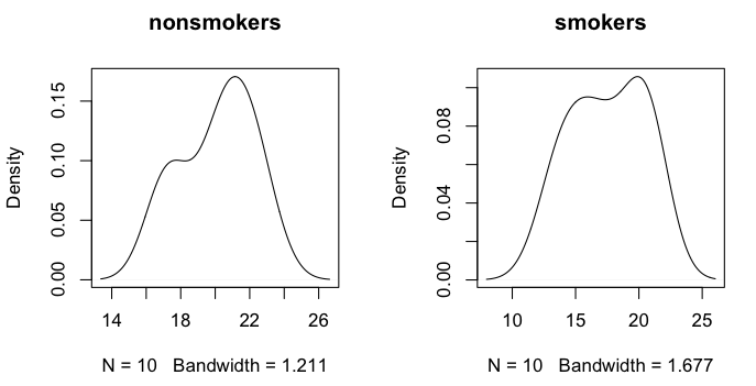
successfully on the digit span task. An examination of the distributions would
be in order at this point, as the t-test assumes sampling from normal parent
populations.
> par(mfrow=c(1,2))               # set graphics window to plot side by side
> plot(density(nonsmokers), main="nonsmokers")
> plot(density(smokers), main="smokers")
The smoothed distributions appear reasonably mound-shaped, although with samples
this small, it's hard to say for sure what the parent distribution looks like.
There may be a wee bit of bimodality.
Another way to examine the data graphically is with side-by-side boxplots.
(NOTE: Close the graphics window before executing the following command, so
that the parameters of the graphics device will be reset.)
> boxplot(nonsmokers, smokers, ylab="Scores on Digit Span Task",     # plot and label y-axis
+         names=c("nonsmokers","smokers"),                           # group names on x-axis
+         main="Digit Span Performance by\n Smoking Status")         # main title
Note: The "\n" inside the main title causes it to be printed on two lines. I'm not
entirely sure this will work in Windows, but it should.
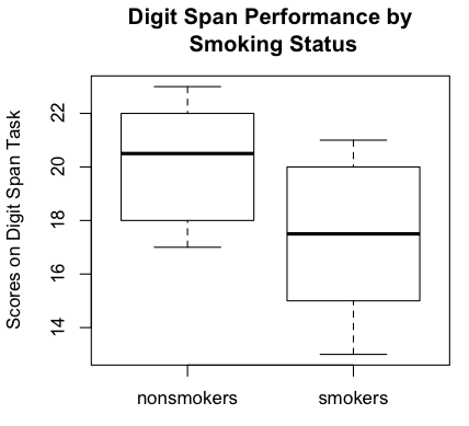
Boxplots are becoming the standard graphical method of displaying this sort
of data (comparison of groups), although I have an issue with the fact that
boxplots are median-oriented graphics, while the t-test is comparing means.
It's easy enough to plot the means inside the boxes, and I'll show you how in
another tutorial. We could also do a
bar graph with error bars (which requires some finagling), and I will discuss
this is a future tutorial, but the bar graph would display less information
about the data. Meanwhile, the boxplots show the nonsmokers to have done better
on the digit span task than the smokers. It also shows an absence of outliers,
which is good news. Of course, the standard numerical summaries could also
be obtained.
> mean(nonsmokers)
[1] 20.1
> sd(nonsmokers)
[1] 2.131770
> mean(smokers)
[1] 17.5
> sd(smokers)
[1] 2.953341
If you want standard errors, there is no built-in function (we will write one
later), but they are easily enough calculated.
> sqrt(var(nonsmokers)/length(nonsmokers))       # assumes no missing values
[1] 0.674125
> sqrt(var(smokers)/length(smokers))             # ditto
[1] 0.9339284
There is little left to do but the statistical test. The t-test can be done either by entering the names of the two groups (or
two numeric vectors) into the t.test() function,
or by using a formula interface if the data are in a data frame (below).
> t.test(nonsmokers, smokers)

	Welch Two Sample t-test

data:  nonsmokers and smokers
t = 2.2573, df = 16.376, p-value = 0.03798
alternative hypothesis: true difference in means is not equal to 0
95 percent confidence interval:
 0.1628205 5.0371795
sample estimates:
mean of x mean of y
     20.1      17.5
By default the two-tailed test is done, and the Welch correction for
nonhomogeneity of variance is applied. Both of these options can easily enough
be changed.
> t.test(nonsmokers, smokers, alternative="greater", var.equal=T)

	Two Sample t-test

data:  nonsmokers and smokers
t = 2.2573, df = 18, p-value = 0.01833
alternative hypothesis: true difference in means is greater than 0
95 percent confidence interval:
 0.6026879       Inf
sample estimates:
mean of x mean of y
     20.1      17.5
The output also includes a 95% CI (change this using "conf.level=") for the
difference between the means, and it includes the sample means. Note that the
t.test()
function always subtracts first group minus second group. Since the "nonsmokers"
were entered first into the function, and our hypothesis was that they would
score higher on the digit span test, this dictated the alternative hypothesis
to be "difference between means is greater than zero." The null hypothesized
difference can also be changed by setting the "mu=" option.
The Formula Interface
I hope you haven't erased those vectors, because now we are going to make a
data frame from them.
> scores = c(nonsmokers, smokers)
> groups = c("nonsmokers","smokers")        # Make sure these are in the right order!
> groups = rep(groups, times=c(10,10))      # 10 nonsmokers, 10 smokers
> mj.data = data.frame(groups, scores)
> mj.data
       groups scores
1  nonsmokers     18
2  nonsmokers     22
3  nonsmokers     21
4  nonsmokers     17
5  nonsmokers     20
6  nonsmokers     17
7  nonsmokers     23
8  nonsmokers     20
9  nonsmokers     22
10 nonsmokers     21
11    smokers     16
12    smokers     20
13    smokers     14
14    smokers     21
15    smokers     20
16    smokers     18
17    smokers     13
18    smokers     15
19    smokers     17
20    smokers     21
> rm(scores, groups)                        # Why is this a good idea?
> attach(mj.data)
Now for some descriptive statistics.
> by(scores, groups, mean)                  # or tapply(scores,groups,mean)
groups: nonsmokers
[1] 20.1
----------------------------------------------------------
groups: smokers
[1] 17.5

> by(scores, groups, sd)
groups: nonsmokers
[1] 2.131770
----------------------------------------------------------
groups: smokers
[1] 2.953341
The boxplot function also accepts a formula interface.
> boxplot(scores ~ groups) # output not shown
Read the formula as "scores by groups". Notice you get group labels on the
x-axis this way, too. The boxplots will be plotted in the order in which R sees
the levels of the groups, which is usually (but not always!) in alphabetical
order. If you want some other order, the factor can be releveled, and I'll
discuss this in a future tutorial.
Finally, the t-test...
> t.test(scores ~ groups)

	Welch Two Sample t-test

data:  scores by groups
t = 2.2573, df = 16.376, p-value = 0.03798
alternative hypothesis: true difference in means is not equal to 0
95 percent confidence interval:
 0.1628205 5.0371795
sample estimates:
mean in group nonsmokers    mean in group smokers
                    20.1                     17.5
Important note: The difference between the means is calculated by subtracting
one group mean from the other, of course, and for the two-tailed (two.sided)
test, it doesn't really matter what order the means are subtracted in. For
directional tests, it does. If you do
levels(mj.data$groups), R will let you in on what
order that is: first listed group minus second listed group. In this case,
that would be nonsmokers' mean minus smokers' mean. Set your
"alternative=" option accordingly.
If you don't care for attaching data frames (and I usually try to avoid it), the
t.test() function also has a "data=" option when used
with the formula interface (but not otherwise).
> detach(mj.data)
> t.test(scores ~ groups, data=mj.data)     ### output not shown
Textbook Problems
Problems in textbooks often leave out the raw data and just present summary
statistics. There is no provision for entering the summary stats into the
t.test() function, so such problems would have to
be calculated at the command prompt.
       Two groups of ten subjects each were given the digit span subtest from
       the Wechsler Adult Intelligence Scale. One group consisted of regular
       smokers of marijuana, while the other group consisted of nonsmokers.
       Below are summary statistics for number of items completed correctly
       on the digit span task. Is there a significant difference between the
       means of the two groups?

             smokers     nonsmokers
             ----------------------
       mean    17.5         20.1
       sd       2.95         2.13

> mean.diff = 17.5 - 20.1
> df = 10 + 10 - 2
> pooled.var = (2.95^2 * 9 + 2.13^2 * 9) / df
> se.diff = sqrt(pooled.var/10 + pooled.var/10)
> t.obt = mean.diff / se.diff
> t.obt
[1] -2.259640
> p.value = 2 * pt(abs(t.obt), df=df, lower.tail=F)        # two-tailed
> p.value
[1] 0.03648139
A custom function could be written if these calculations had to be done
repeatedly, but (STUDENTS!) there is a certain educational value to be had from
doing them by hand!
Power
The power.t.test() function has the following
syntax (from the help page for this function).
power.t.test(n = NULL, delta = NULL, sd = 1, sig.level = 0.05, power = NULL,
             type = c("two.sample", "one.sample", "paired"),
             alternative = c("two.sided", "one.sided"),
             strict = FALSE)
Exactly one of the options on the first line should be set to "NULL", and R will
then calculate it from the remaining values. Suppose we wanted a power of 85%
for the Scott Keats experiment, and were anticipating a mean difference of 2.5
and a pooled standard deviation of 2.6. How many subjects should be used per
group if a two-tailed test is planned?
> power.t.test(delta=2.5, sd=2.6, sig.level=.05, power=.85,     # n=NULL by default
+              type="two.sample", alternative="two.sided")

     Two-sample t test power calculation

              n = 20.43001
          delta = 2.5
             sd = 2.6
      sig.level = 0.05
          power = 0.85
    alternative = two.sided

 NOTE: n is number in *each* group
So there you go: to play it safe, 21 subjects per group should be used.
Homogeneity of Variance
The standard, textbook, pooled-variance t-test assumes homogeneity of
variance. The easiest way to deal with nonhomogeneity of variance is to allow
R to do what it does by default anyway--run the t-test using the Welch
correction for nonhomogeneity. Further discussion of nonhomogeneity of variance
will occur in the ANOVA tutorial.
I'm not entirely happy that nonhomogeneity is assumed by default and then
"swept under the rug" by applying the Welch correction. If the variances are
different, that could be an interesting effect in itself. In any event, I don't
think it should just be ignored. In my opinion, the pooled-variance t-test
should be the default. But then, they didn't ask me.
Alternatives to the t Test
If the normality assumption of the t-test is violated, and the sample sizes
are two small to heal that via an appeal to the central limit theorem, then a
nonparametric alternative test should be sought. The standard alternative to the
independent samples t-test is what we old timers were taught to call the
Mann-Whitney U test. For some reason, this name is now out of fashion, and the
test goes by the name Wilcoxin-Mann-Whitney test, or Wilcoxin rank sum test,
or some variant thereof. The syntax is very similar, and it will work with or
without the formula interface.
> wilcox.test(nonsmokers, smokers)     # if these vectors are still in your workspace

	Wilcoxon rank sum test with continuity correction

data:  nonsmokers and smokers
W = 76.5, p-value = 0.04715
alternative hypothesis: true location shift is not equal to 0

Warning message:
In wilcox.test.default(nonsmokers, smokers) :
  cannot compute exact p-value with ties

>    ### and now the formula interface...
> wilcox.test(scores ~ groups, data=mj.data)

	Wilcoxon rank sum test with continuity correction

data:  scores by groups
W = 76.5, p-value = 0.04715
alternative hypothesis: true location shift is not equal to 0

Warning message:
In wilcox.test.default(x = c(18, 22, 21, 17, 20, 17, 23, 20, 22,  :
  cannot compute exact p-value with ties
The test assumes continuous variables without ties (neither of which is the case
here).
revised 2016 January 30
| Table of Contents
| Function Reference
| Function Finder
| R Project |
|