
| Table of Contents
| Function Reference
| Function Finder
| R Project |
DATA FRAMES
Preamble and Editorial
There is plenty to say about data frames because they are the primary data
structure in R. Some of what follows is essential knowledge. Some of it will be
satisfactorily learned for now if you remember that "R can do that." I will try
to point out which parts are which. Set aside some time. This is a long one! If
you break this one up into multiple sessions, always save your workspace when
you quit.
> setwd("Rspace")                      # if you have this directory
> rm(list=ls())                        # clear the workspace
A Note About Data Management. We can hardly discuss data frames without talking
about data management. How do you get your data in? How do you edit them once
they're in? I'm sorry to report that this is one area in which R is particularly
poor. The facilities in R for data management are, to say the least, clumsy and
inadequate. On top of that, there doesn't seem to be any move afoot to
improve them.
If I were a programmer, this is where I'd be working to improve R. The single
most common "excuse" I've heard from people for not adopting R is lack of data
management tools. Now don't get me wrong. R does contain very powerful data
management tools, and you can accomplish just about any data management task
from within R. It's just not the way most people want to work with their data.
Most people (so they tell me anyway) find a command line interface a clumsy way
to manipute a (large) data set. I get that.
People working with other statistics software packages are used to a
spreadsheet-like interface for entering and editing data. I've worked with that
interface in SPSS, and I personally find it clunky and awkward. I'd much rather
use a modern spreadsheet to manage my data, and that's what I do in R. For some
reason, other people want the spreadsheet interface integrated, even if it's
"clunky and awkward."
R does have a spreadsheet-like data editor. It is invoked by functions such
as edit(), fix(), data.entry(), and maybe a couple
others. I don't use these functions, and I'm not going to discuss them. Here's
why. They just flat out don't work on my system. They're not awkward or clumsy,
they generate error messages! I am at the moment sitting beside a Windows XP
computer running R 3.1.2, and the functions are working there, but they
are awkward and illogical. So even when these data management functions do work,
they are just not convenient (or particularly safe!) ways to manage data.
Bottom line--you are probably going to end up using a spreadsheet or some
other third-party software to manage larger data sets. I will show you a
little of how to do that in this tutorial and the next one. I should also
say that R can be set up to work with data base management software such as
SQL, whatever that is. I don't know how to do that, and I've read mixed
reviews of its effectiveness. It also sounds like you better be running
Windows if you want to make it work, but I haven't really looked into it,
and don't plan to. Final note: R keeps data in RAM, so if you plan to work
with really, really large data sets, you're going to have to interact with
some sort of data base software, or have lots and lots of RAM. I have 4 GB
in my system and have worked with data sets that have tens of thousands of
cases and scores of variables. Having all the data in RAM makes R very fast.
However, available RAM is the limiting
factor in how large a data set you can work with entirely within R.
Definition and Examples (essential)
A data frame is a table, or two-dimensional array-like structure, in which
each column contains measurements on one variable, and each row contains one
case. As we shall see, a "case" is not necessarily the same as an experimental
subject or unit, although they are often the same. Technically, in R a data
frame is a list of column vectors, although there is only one reason why you
might need to remember such an arcane thing. Unlike an array, the data you
store in the columns of a data frame can be of various types. I.e., one column
might be a numeric variable, another might be a factor, and a third might be
a character variable. All columns have to be the same length (contain the same
number of data items, although some of those data items may be missing values).
Let's say we've collected data on one response variable or DV from 15
subjects, who were divided into three experimental groups called control
("contr"), treatment one ("treat1"), and treatment two ("treat2"). We might be
tempted to table the data as follows.
contr     treat1    treat2
---------------------------
  22        32        30
  18        35        28
  25        30        25
  25        42        22
  20        31        33
---------------------------
While this is a perfectly acceptable table, it is NOT a data frame, because
values on our one response variable have been divided into three columns (and so
have values on the grouping or independent variable). A data frame has the name
of the variable at the top of the column, and values of that variable in the
column under the variable name. So the data above should be tabled as follows.
scores     group
----------------
  22       contr
  18       contr
  25       contr
  25       contr
  20       contr
  32      treat1
  35      treat1
  30      treat1
  42      treat1
  31      treat1
  30      treat2
  28      treat2
  25      treat2
  22      treat2
  33      treat2
----------------
This is a proper data frame. It does not matter in what
order the columns appear, as long as each column contains values of one
variable, and every recorded value of that variable is in that column.
In a previous tutorial we used the data object "women" as an example of a
data frame.
> women
   height weight
1      58    115
2      59    117
3      60    120
4      61    123
5      62    126
6      63    129
7      64    132
8      65    135
9      66    139
10     67    142
11     68    146
12     69    150
13     70    154
14     71    159
15     72    164
In this data frame we have two numeric variables and no real explanatory
variables (IVs) or response variables (DVs). Notice when R prints out a data
frame, it numbers the rows. These numbers are for convenience only and are not
part of the data, and I'll have much more to say about them shortly.
We can refer to any value, or subset of values, in this data frame using the
already familiar notation.
> women[12,2]                          # row 12, column 2; note the square brackets
[1] 150
> women[8,]                            # row 8, all columns (blank index means "all")
  height weight
8     65    135
> women[1:5,]                          # rows 1 through 5, all columns
  height weight
1     58    115
2     59    117
3     60    120
4     61    123
5     62    126
> women[,2]                            # all rows, column 2
 [1] 115 117 120 123 126 129 132 135 139 142 146 150 154 159 164
> women[c(1,3,7,13),]                  # rows 1, 3, 7, and 13, all columns
   height weight
1      58    115
3      60    120
7      64    132
13     70    154
> women[c(1,3,7,13),1]                 # rows 1, 3, 7, and 13, column 1
[1] 58 60 64 70
Here's the catch. Those index numbers do NOT necessarily correspond to the
numbers you see printed at the left of the data frame. This can be confusing,
and it is something you need to keep in mind. I will explain in a moment.
Another built-in data object that is a data frame is "warpbreaks". This data
frame contains 54 cases, so I will print out only every third one. I do this
with the sequence function, since this function creates a vector just as the
c() function did in the above examples.
> warpbreaks[seq(from=1, to=54, by=3),]
   breaks wool tension
1      26    A       L
4      25    A       L
7      51    A       L
10     18    A       M
13     17    A       M
16     35    A       M
19     36    A       H
22     18    A       H
25     28    A       H
28     27    B       L
31     19    B       L
34     41    B       L
37     42    B       M
40     16    B       M
43     21    B       M
46     20    B       H
49     17    B       H
52     15    B       H
In this data frame we have one numeric variable (number of breaks), and two
categorical variables (type of wool and tension on the wool). We don't have to
look at the data frame itself to get this information. We can also use the
str() function, which displays a breakdown of
the structure of a data frame (or other data object).
> str(warpbreaks)
'data.frame':   54 obs. of  3 variables:
 $ breaks : num  26 30 54 25 70 52 51 26 67 18 ...
 $ wool   : Factor w/ 2 levels "A","B": 1 1 1 1 1 1 1 1 1 1 ...
 $ tension: Factor w/ 3 levels "L","M","H": 1 1 1 1 1 1 1 1 1 2 ...
Here are two more handy functions for finding out what's in a data frame.
> head(warpbreaks)                     # see the first six rows of data
  breaks wool tension
1     26    A       L
2     30    A       L
3     54    A       L
4     25    A       L
5     70    A       L
6     52    A       L
> summary(warpbreaks)                  # see a summary of each of the variables
     breaks      wool   tension
 Min.   :10.00   A:27   L:18
 1st Qu.:18.25   B:27   M:18
 Median :26.00          H:18
 Mean   :28.15
 3rd Qu.:34.00
 Max.   :70.00
Another example is the data object "sleep".
> sleep
   extra group ID
1    0.7     1  1
2   -1.6     1  2
3   -0.2     1  3
4   -1.2     1  4
5   -0.1     1  5
6    3.4     1  6
7    3.7     1  7
8    0.8     1  8
9    0.0     1  9
10   2.0     1 10
11   1.9     2  1
12   0.8     2  2
13   1.1     2  3
14   0.1     2  4
15  -0.1     2  5
16   4.4     2  6
17   5.5     2  7
18   1.6     2  8
19   4.6     2  9
20   3.4     2 10
Here we have two variables, the change in sleep time a subject got ("extra"),
and what drug the subject received ("group"). There is also a subject identifier
(ID), indicating that the first 10 cases and last 10 cases are the same subjects.
In this data frame, the first variable
(the dependent variable, DV, response variable, etc.) is numeric and the
second (the independent variable, IV, explanatory variable, grouping variable,
etc.) is categorical, even though the categorical variable is coded as a
number. Once again, it does not matter in what order the columns occur. Put the
IV in the first column, the DV in the third column, and the subject ID between
them, if you want.
However, if categorical variables are coded as numbers (a common practice),
R will not know this until you tell it. Has R been told that "group" is a factor
in this data frame? The str() is one handy way to
find out.
> str(sleep)
'data.frame':	20 obs. of  3 variables:
 $ extra: num  0.7 -1.6 -0.2 -1.2 -0.1 3.4 3.7 0.8 0 2 ...
 $ group: Factor w/ 2 levels "1","2": 1 1 1 1 1 1 1 1 1 1 ...
 $ ID   : Factor w/ 10 levels "1","2","3","4",..: 1 2 3 4 5 6 7 8 9 10 ...
In this case, the fact that "group" is a factor is stored internally in the
data frame, but that will not always be the case. So it's worth taking a look
to make sure things you intend to be factors are being interpreted as
factors by R. You can do this with str(),
but you can also do it with summary(),
because numeric variables and factors are summarized differently.
> summary(sleep)
     extra        group        ID
 Min.   :-1.600   1:10   1      :2
 1st Qu.:-0.025   2:10   2      :2
 Median : 0.950          3      :2
 Mean   : 1.540          4      :2
 3rd Qu.: 3.400          5      :2
 Max.   : 5.500          6      :2
                         (Other):8
Notice that numeric variables ("extra") are summarized with numerical summary
statistics, while factors are summarized with a frequency table. In these data,
there are 10 subjects in group 1 and 10 subjects in group 2. There are also
two subjects with ID 1, two subjects with ID 2, etc.
An Ambiguous Case (essential)
Entering data into a data frame sometimes involves making a tough decision as
to what your variables are. The following example is from a built-in data object
called "anorexia". This data set is not in the libraries that are loaded by
default when R starts, so to see it, the first thing we need to do is attach the
correct library to the search path. Let's see how that works.
> search()
 [1] ".GlobalEnv"        "tools:RGUI"        "package:stats"
 [4] "package:graphics"  "package:grDevices" "package:utils"
 [7] "package:datasets"  "package:methods"   "Autoloads"
[10] "package:base"
This is the default search path, the one you have right after R starts. (It
will be a little different in different operating systems.) We want to see an
object in the MASS library (or package), which is not currently in the search
path. So to get it into the search path, do this.
> library(MASS)
> search()
 [1] ".GlobalEnv"        "package:MASS"      "tools:RGUI"
 [4] "package:stats"     "package:graphics"  "package:grDevices"
 [7] "package:utils"     "package:datasets"  "package:methods"
[10] "Autoloads"         "package:base"
Notice we have added "package:MASS" to the search path in position 2. This means
if we request an R object, R will look first in the global environment (the
workspace), and if the object is not found there, R will look next in MASS, then
in RGUI, then in stats, and so on, until the object either is found or R runs
out of places to look for it. The "anorexia" data frame is 72 cases long, so to
conserve space we will look at only every fifth row of it.
> data(anorexia)                       # put a copy in your workspace
> anorexia[seq(from=1, to=72, by=5),]
   Treat Prewt Postwt
1   Cont  80.7   80.2
6   Cont  88.3   78.1
11  Cont  77.6   77.4
16  Cont  77.3   77.3
21  Cont  85.5   88.3
26  Cont  89.0   78.8
31   CBT  79.9   76.4
36   CBT  80.5   82.1
41   CBT  70.0   90.9
46   CBT  84.2   83.9
51   CBT  83.3   85.2
56    FT  83.8   95.2
61    FT  79.6   76.7
66    FT  81.6   77.8
71    FT  86.0   91.7
The data frame contains data from women who underwent treatment for anorexia. In
the first column we have the treatment variable ("Treat"). The second column
contains the pretreatment body weight in pounds ("Prewt"). The third column
contains the posttreatment body weight in pounds ("Postwt"). So where is the
ambiguity?
Here's the awkward question. In our analysis of these data, do we wish to
treat weight as two variables ("Prewt" and "Postwt") each measured once on each
subject, or as one variable (call it "weight") measured twice on each subject?
The data frame is currently arranged as if the plan was for an analysis of
covariance, with "Postwt" being the response, "Treat" the explanatory variable,
and "Prewt" the covariate. Prewt and Postwt are treated as two variables.
If the plan was for a repeated measures ANOVA, then the data frame is wrong,
because in this case, "weight" is ONE variable measured twice ("pre" and "post")
on each woman. In this analysis, we would also need to add a "subject" identifier
to the data frame as well, since each subject would have two lines, a "pre" line
and a "post" line. (NOTE: There is an optional package that can be downloaded
from CRAN which will do repeated measures ANOVA on data in this format.
Google EZANOVA for details. The package is called ez.)
It's not a disaster. The data frame is easy enough to rearrange on the fly,
and we will do so below.
FYI, this is how we get the MASS package out of the search path if
we no longer need it, which we don't. (Don't remove "anorexia" from your
workspace, however.)
> detach("package:MASS")
Creating a Data Frame in R (essential)
The easiest way--and the usual way--of getting a data frame into the R
workspace is to read it in from a file. We will do that below (a few sections
from now).
Sometimes it becomes necessary to create one at the console, however. Here are
the steps involved:
- Type each variable into a vector.
- Use the data.frame() function to
create a data frame from the vectors.
You may remember these data from the "Objects" tutorial.
name     age  hgt  wgt  race year   SAT
Bob       21   70  180  Cauc   Jr  1080
Fred      18   67  156 Af.Am   Fr  1210
Barb      18   64  128 Af.Am   Fr   840
Sue       24   66  118  Cauc   Sr  1340
Jeff      20   72  202 Asian   So   880
Let's make a data frame of this. The method used here is a somewhat unforgiving
method of entering data. I will make an intentional mistake and show you how to
correct it below. However, the values for each of the variables have to remain
aligned. I.e., Bob is age 21, 70 in. tall, weighs 180 lbs., etc. If you get the
data values out of order in any given vector, or if you leave one out, for now
all I can say is, "Start again!"
> ls()
[1] "anorexia"
> name = scan(what="character")
1: Bob Fred Barb Sue Jeff         # Remember: press Enter twice to end data entry.
6:
Read 5 items
> age = scan()
1: 21 18 18 24 20
6:
Read 5 items
> hgt = scan()
1: 70 67 64 66 72
6:
Read 5 items
> wgt = scan()                    # I am making a mistake intentionally here.
1: 180 156 128 1118 202
6:
Read 5 items
> race = scan(what="character")   # One value here is being recorded as missing, NA.
1: Cauc Af.Am NA Cauc Asian
6:
Read 5 items
> year = scan(what="character")
1: Jr Fr Fr Sr So
6:
Read 5 items
> SAT = scan()                    # One value here is being recorded as missing, NA.
1: 1080 1210 840 NA 880
6:
Read 5 items
> my.data = data.frame(name, age, hgt, wgt, race, year, SAT)
> my.data
  name age hgt  wgt  race year  SAT
1  Bob  21  70  180  Cauc   Jr 1080
2 Fred  18  67  156 Af.Am   Fr 1210
3 Barb  18  64  128  <NA>   Fr  840
4  Sue  24  66 1118  Cauc   Sr   NA
5 Jeff  20  72  202 Asian   So  880
Tah dah! It's as "simple" as that. You wouldn't want to have to do that with a
large data set, however, and that's why we'll learn how to read them in from a
file. DON'T clean up your workspace. We will carry this
example over into the next section.
> ls()                            # Messy! But leave it that way for now.
[1] "age"      "anorexia" "hgt"      "my.data"  "name"     "race"
[7] "SAT"      "wgt"      "year"
Accessing Information Inside a Data Frame (essential)
First, let's look at a few functions that allow us to get general
information about a data frame...
> dim(my.data)                    # Get size in rows by columns.
[1] 5 7
> names(my.data)                  # Get the names of variables in the data frame.
[1] "name" "age"  "hgt"  "wgt"  "race" "year" "SAT"
> str(my.data)                    # See the internal structure of the data frame.
'data.frame':	5 obs. of  7 variables:
 $ name: Factor w/ 5 levels "Barb","Bob","Fred",..: 2 3 1 5 4
 $ age : num  21 18 18 24 20
 $ hgt : num  70 67 64 66 72
 $ wgt : num  180 156 128 1118 202
 $ race: Factor w/ 3 levels "Af.Am","Asian",..: 3 1 NA 3 2
 $ year: Factor w/ 4 levels "Fr","Jr","So",..: 2 1 1 4 3
 $ SAT : num  1080 1210 840 NA 880
These are self-explanatory, with the exception of
str(). First, notice that our character
variables were entered into the data frame as factors. This is standard in R,
but it may not be what you want. Second, notice on the lines giving info about
factors that there are strange numbers at the ends of those lines. You don't
have to worry about these. What R is telling you is that factors are coded
internally in R as numbers. R will keep it all straight for you, so don't
sweat the details.
The summary() function is VERY useful here.
> summary(my.data)
   name        age            hgt            wgt            race   year
 Barb:1   Min.   :18.0   Min.   :64.0   Min.   : 128.0   Af.Am:1   Fr:2
 Bob :1   1st Qu.:18.0   1st Qu.:66.0   1st Qu.: 156.0   Asian:1   Jr:1
 Fred:1   Median :20.0   Median :67.0   Median : 180.0   Cauc :2   So:1
 Jeff:1   Mean   :20.2   Mean   :67.8   Mean   : 356.8   NA's :1   Sr:1
 Sue :1   3rd Qu.:21.0   3rd Qu.:70.0   3rd Qu.: 202.0
          Max.   :24.0   Max.   :72.0   Max.   :1118.0

      SAT
 Min.   : 840
 1st Qu.: 870
 Median : 980
 Mean   :1002
 3rd Qu.:1112
 Max.   :1210
 NA's   :1
Let's take a look. There is a variable called "name", which R is summarizing
as a factor. We probably don't really want that, because it's not a grouping
variable, but for now no harm no foul. There is a variable called "age",
which is numeric, a variable called "hgt", which is numeric, and a variable
called "wgt", which is numeric. Do you see any problems here?
The "age" and "hgt" variables look entirely reasonable as far as min and
max values are concerned, but wgt does not. Maximum wgt is 1118 lbs. Really?
Something clearly went wrong here, and we are going to have to track it down
and fix it!
The variables "race" and "year" are factors or categorical variables. See
any problems? Yes, there is a missing value (NA) in "race" that didn't occur
in the original data table. Something else we're going to have to fix.
Finally, "SAT", also numeric, has a missing value that we are going to have
to track down. This is the advantage of using summary().
It shows which variables have values missing, and you can look at the
range of the numeric variables and see if there is anything suspicious, like a
body weight of 1118 lbs.
There are four ways to get at the data inside a data frame, and this is NOT
one of them.
> SAT
[1] 1080 1210  840   NA  880
That only seemed to work, because remember when you created the data frame, you
started by putting a vector called "SAT" into the workspace. THAT'S what you're
seeing now! You are NOT seeing the SAT variable from inside the data frame.
R looks in your workspace FIRST, so that is the "SAT" that it came up with.
Confusing, right? So that we don't remain confused, let's erase all those
vectors EXCEPT "age", which we will keep to illustrate
something that you will need to remember about R.
> ls()
[1] "age"      "anorexia" "hgt"      "my.data"  "name"     "race"
[7] "SAT"      "wgt"      "year"
> rm(hgt, name, race, SAT, wgt, year)       ##### DON'T erase my.data!
> ls()
[1] "age"      "anorexia" "my.data"
Now if we try to see SAT as we did above...
> SAT
Error: object 'SAT' not found
...we get an error. R will not look inside data frames for variables unless
you tell it to. Here are the four ways to do that.
- by using $
- by using with()
- by using data=
- by using attach()
A data frame is a list of column vectors. We can extract items from inside
it by using the usual list indexing device, $. To do this, type the name of the
data frame, a dollar sign, and the name of the variable you want to work
with. You can leave spaces around the $ if you want to. Or not.
> my.data $ SAT
[1] 1080 1210  840   NA  880
> my.data$SAT
[1] 1080 1210  840   NA  880
This can certainly be a nuisance, because it will mean that in some commands
you have to type the data frame name multiple times. An example is the command
that calculates a correlation.
> cor(my.data$hgt, my.data$wgt)
[1] -0.2531835
In this case, you can use the with() function
to tell R where to get the data.
> with(my.data, cor(hgt, wgt))    # syntax: with(dataframe.name, function(arguments))
[1] -0.2531835
It doesn't save much typing in this example, but there are cases where that will
save a LOT of typing! Notice the syntax of this function. You type the name of
the data frame first, followed by a comma, followed by the function you want
to execute, then you close the parentheses on with().
As we will learn later, some functions, especially significance tests, take
what's called a formula interface. When that's the case, there is (almost) always
a data= option to specify the name of the data frame where the variables are to be
found. I'll just show you an example for now. We'll have plenty of time to
examine the formula interface later. For now, all you need to be aware of is the
tilde, which is always present in a formula. In this case, the formula starts
with the tilde (the squiggly line), which is unusual.
> cor.test( ~ hgt + wgt, data=my.data)      #syntax: function(formula, data=dataframe.name)

        Pearson's product-moment correlation

data:  hgt and wgt
t = -0.4533, df = 3, p-value = 0.6811
alternative hypothesis: true correlation is not equal to 0
95 percent confidence interval:
 -0.9281289  0.8100218
sample estimates:
       cor
-0.2531835
Finally, there is the dreaded attach()
function. This attaches the data frame to your search path (in position 2) so
that R will know to look there for data objects that are referenced by name.
Some people use this device routinely when working with data frames, but it
can cause problems, and we are about to see one.
> attach(my.data)
The following object(s) are masked _by_ .GlobalEnv :

    age
Say what? When an object is masked (or shadowed) by the global environment,
that means there is a data object in the workspace that has this name AND
there is a variable inside the data frame that has this name. I can now ask
directly for any variable inside the data frame EXCEPT age.
> SAT                             # same as my.data$SAT (well, almost)
[1] 1080 1210  840   NA  880
> mean(wgt)                       # same as mean(my.data$wgt)
[1] 356.8
> table(year)                     # same as table(my.data$SAT)
year
Fr Jr So Sr
 2  1  1  1
> age
[1] 21 18 18 24 20
You might think you are seeing my.data$age here, but YOU ARE NOT! You're seeing
"age" from the workspace, BECAUSE THAT'S WHERE R LOOKS FIRST. In this case,
both copies of "age" are the same, but that won't always be true.
> age = 112                       # modifies the first copy it finds
> age
[1] 112
> my.data$age
[1] 21 18 18 24 20
The assignment changed the value of "age" in the workspace, because that is
the first "age" R saw, but did not change the value of "age" in the data frame.
If we remove age from the workspace, R will then search inside the data frame
for it, because the data frame is attached in position 2 of the search path.
> rm(age)
> age
[1] 21 18 18 24 20
The lesson is, when you get one of these masking (or shadowing) conflicts,
WATCH OUT! Be extra careful to know which version of the variable you're
working with. This has tripped up many an R user, including me. This is why
you want to keep your workspace as clean as possible. The best strategy here
is to remove the masking variable from the workspace. If you want to keep it,
at least rename it and then remove the conflicting version from the workspace.
You'll eventually be sorry if you don't!
One more lesson...
> detach(my.data)
When you're done with an attached data frame, ALWAYS detach it. This will
remove it from the search path so that R will no longer look inside it for
variables. You'll have to go back to using $ to reference variables inside the
data frame after it is detached. This isn't necessary if you're going to quit
your R session right away. Quitting detaches everything that was attached. But
if you're going to continue working, detach data frames you no longer need.
Otherwise, your search path will get messy, and you'll get more and more
masking conflicts as other objects are attached.
DON'T erase my.data. We still need it.
Data Frame Indexing and Row Names (critical)
This will cost you BIGTIME eventually if you don't pay close attention!
This drove me nuts for awhile until I figured out what was happening.
> ls()                            # Still there?
[1] "anorexia" "my.data"
> my.data
  name age hgt  wgt  race year  SAT
1  Bob  21  70  180  Cauc   Jr 1080
2 Fred  18  67  156 Af.Am   Fr 1210
3 Barb  18  64  128  <NA>   Fr  840
4  Sue  24  66 1118  Cauc   Sr   NA
5 Jeff  20  72  202 Asian   So  880
Let's talk about those line numbers at the leftmost verge of the printed data
frame. THEY ARE NOT NUMBERS. Let me repeat that. THEY ARE NOT NUMBERS. They are
row names. They are character values. So the rows and columns of this data
frame are NAMED as follows:
> dimnames(my.data)
[[1]]
[1] "1" "2" "3" "4" "5"

[[2]]
[1] "name" "age"  "hgt"  "wgt"  "race" "year" "SAT"
What's the big deal?
Look at the printed data frame. Suppose we wanted to extract Barb's weight.
That's the value in row 3 and column 4, so we could get it this way.
> my.data[3,4]                    # Remember to use square brackets for indexing.
[1] 128
"Yeah, so?" We could also get it this way...
> my.data[3,"wgt"]
[1] 128
...and this way...
> my.data["3","wgt"]
[1] 128
Those last two ways seem to be the same, BUT THEY ARE NOT!!!
Let's sort the data frame using the age variable. Sorting a data frame is
done using the order() function. Remember how
it worked when we sorted a vector? If a call to the
order() function is put in place of the row
index, the data frame will be sorted on whatever variable is specified inside
that function. You will have to use the full name of the variable; i.e., you
will have to use the $ notation. (Why?) Otherwise, R will be looking in your
workspace for a variable called "age", not finding it, and giving a "not
found" error. It happens to me a lot, so you might as well just get used to it!
> my.data[order(my.data$age),]
  name age hgt  wgt  race year  SAT
2 Fred  18  67  156 Af.Am   Fr 1210
3 Barb  18  64  128 Af.Am   Fr  840
5 Jeff  20  72  202 Asian   So  880
1  Bob  21  70  180  Cauc   Jr 1080
4  Sue  24  66 1118  Cauc   Sr 1340
Observe the row names! They have also been sorted, haven't they? Let's save
this into a new data object so we can play with it a bit.
> my.data[order(my.data$age),] -> my.data.sorted      # Did you remember up arrow?
> my.data.sorted
  name age hgt  wgt  race year  SAT
2 Fred  18  67  156 Af.Am   Fr 1210
3 Barb  18  64  128 Af.Am   Fr  840
5 Jeff  20  72  202 Asian   So  880
1  Bob  21  70  180  Cauc   Jr 1080
4  Sue  24  66 1118  Cauc   Sr 1340
Now let's try to extract Barb's weight from this new data frame.
> my.data.sorted[3,4]                  ### Wrong!
[1] 202
> my.data.sorted[3,"wgt"]              ### Also wrong!
[1] 202
> my.data.sorted["3","wgt"]            ### Correct!
[1] 128
> my.data.sorted[2,4]                  ### Also correct!
[1] 128
Confused yet?
Here's what you have to remember. Those numbers that often print out on the
left side of a data frame ARE NOT NUMBERS. They're row names--character values.
So data frames
have both row and column names, whether you like it or not! The point becomes
clearer when we give the rows actual names. Let's erase the names from my.data
and then re-enter them as row names.
> rm(my.data.sorted)                   # Get rid of that first.
> my.data$name = NULL                  # This is how you erase a variable from a data frame.
> my.data
  age hgt  wgt  race year  SAT
1  21  70  180  Cauc   Jr 1080
2  18  67  156 Af.Am   Fr 1210
3  18  64  128  <NA>   Fr  840
4  24  66 1118  Cauc   Sr   NA
5  20  72  202 Asian   So  880
> rownames(my.data) = c("Bob","Fred","Barb","Sue","Jeff")
> my.data
     age hgt  wgt  race year  SAT
Bob   21  70  180  Cauc   Jr 1080
Fred  18  67  156 Af.Am   Fr 1210
Barb  18  64  128  <NA>   Fr  840
Sue   24  66 1118  Cauc   Sr   NA
Jeff  20  72  202 Asian   So  880
> my.data["Barb", "wgt"]               # Makes getting Barb's weight a lot easier!
[1] 128
Notice the numbers are gone now because we have actual row names. And OF COURSE
they sort with the rest of the data frame, just as the "number" row names did
above.
> my.data[order(my.data$age),]
     age hgt  wgt  race year  SAT
Fred  18  67  156 Af.Am   Fr 1210
Barb  18  64  128  <NA>   Fr  840
Jeff  20  72  202 Asian   So  880
Bob   21  70  180  Cauc   Jr 1080
Sue   24  66 1118  Cauc   Sr   NA
It would be absolutely silly if they didn't! Just remember: Data frames ALWAYS
have row names. Sometimes those row names just happen to look like numbers.
It's the row names that print out to your console when you ask to see the
data frame, or any part of it, and NOT the index numbers. (R Studio shows you
both when you ask to View a data frame.)
(NOTE: All row names have to be unique. You can't have two Barbs, for
obvious reasons.)
Don't remove my.data yet. We still need it.
Modifying a Data Frame (pretty important)
Rule number one with a bullet:
- NEVER MODIFY AN ATTACHED DATA FRAME!
While this isn't strictly against the law, it's a bad idea and can get very
confusing as to exactly what it is you've modified. I could try to explain it,
but I'm not sure I understand it myself. So just don't do it! (An attached
data frame is a copy of the data frame in the workspace, not the actual data
frame in the workspace. Modifications will be made to the actual data frame in
the workspace, but not to the attached copy.)
The time will come when you want to change a data frame in some way. Here are
some examples of how to do that. You may have noticed that Sue (in the my.data
data frame) is a wee bit on the chunky side. This was an innocent mistake. I
really didn't do that on purpose. How do we fix it? The value was supposed to
be 118, but let's change it to 135 just for kicks.
> ls()                                 # Still there?
[1] "my.data"
> my.data
     age hgt  wgt  race year  SAT
Bob   21  70  180  Cauc   Jr 1080
Fred  18  67  156 Af.Am   Fr 1210
Barb  18  64  128  <NA>   Fr  840
Sue   24  66 1118  Cauc   Sr   NA
Jeff  20  72  202 Asian   So  880
> my.data["Sue", "wgt"] = 135
> my.data
     age hgt wgt  race year  SAT
Bob   21  70 180  Cauc   Jr 1080
Fred  18  67 156 Af.Am   Fr 1210
Barb  18  64 128  <NA>   Fr  840
Sue   24  66 135  Cauc   Sr   NA
Jeff  20  72 202 Asian   So  880
That's all there is to it. Use any kind of indexing you like. Let's use
numerical indexing to give Sue her correct weight, and while we're at it,
let's fix those missing values, too.
> my.data[4,3] = 118
> my.data[3, "race"] = "Af.Am"
> my.data["Sue", 6] = 1340
> my.data
     age hgt wgt  race year  SAT
Bob   21  70 180  Cauc   Jr 1080
Fred  18  67 156 Af.Am   Fr 1210
Barb  18  64 128 Af.Am   Fr  840
Sue   24  66 118  Cauc   Sr 1340
Jeff  20  72 202 Asian   So  880
Just remember that "wgt" is now in column 3, since the row names don't count
as a column.
Now, I have a confession to make. I neglected to detach my.data before I
made those changes. Here are the consequences.
> SAT                             # sees the attached copy
[1] 1080 1210  840   NA  880
> my.data$SAT                     # sees the copy in the workspace
[1] 1080 1210  840 1340  880
> wgt
[1]  180  156  128 1118  202
> race
[1] Cauc  Af.Am <NA>  Cauc  Asian
Levels: Af.Am Asian Cauc
Ack! The attached copy has not been changed. But the copy in the workspace
has been changed. Here's the fix. (Won't work if you weren't as stupid as I
was and didn't have my.data attached while you were making those modifications.)
> detach(my.data)                 # will just give an error if not attached
> attach(my.data)                 # previous attached copy tossed; new attached copy created
> SAT
[1] 1080 1210  840 1340  880
> detach(my.data)
I have to warn you about modifying data frames. It's always a good idea to
make a backup copy in the workspace first. Because there are some commands that
modify data frames that, if they go wrong, can really screw things up! But
let's live dangerously. Suppose we wanted "wgt" to be in kilograms instead of
pounds. Easy enough...
> my.data$wgt / 2.2
[1] 81.81818 70.90909 58.18182 53.63636 91.81818
> my.data                                # Nothing has changed yet. Why not?
     age hgt wgt  race year  SAT
Bob   21  70 180  Cauc   Jr 1080
Fred  18  67 156 Af.Am   Fr 1210
Barb  18  64 128 Af.Am   Fr  840
Sue   24  66 118  Cauc   Sr 1340
Jeff  20  72 202 Asian   So  880
> my.data$wgt / 2.2 -> my.data$wgt       # Aha! It has to be stored back into my.data.
> my.data
     age hgt      wgt  race year  SAT
Bob   21  70 81.81818  Cauc   Jr 1080
Fred  18  67 70.90909 Af.Am   Fr 1210
Barb  18  64 58.18182 Af.Am   Fr  840
Sue   24  66 53.63636  Cauc   Sr 1340
Jeff  20  72 91.81818 Asian   So  880
> my.data$wgt = round(my.data$wgt, 1)    # A little rounding for good measure.
> my.data
     age hgt  wgt  race year  SAT
Bob   21  70 81.8  Cauc   Jr 1080
Fred  18  67 70.9 Af.Am   Fr 1210
Barb  18  64 58.2 Af.Am   Fr  840
Sue   24  66 53.6  Cauc   Sr 1340
Jeff  20  72 91.8 Asian   So  880
Now that we've rounded them off, we've lost the original weight data in
pounds.
> my.data$wgt * 2.2
[1] 179.96 155.98 128.04 117.92 201.96
We could have avoided this by making a backup copy of my.data first, or by
putting the new weight in kilograms into a new column in the data frame.
Let's see how to create a new column in the data frame.
> my.data$IQ = c(115, 122, 100, 144, 96)
> my.data
     age hgt  wgt  race year  SAT  IQ
Bob   21  70 81.8  Cauc   Jr 1080 115
Fred  18  67 70.9 Af.Am   Fr 1210 122
Barb  18  64 58.2 Af.Am   Fr  840 100
Sue   24  66 53.6  Cauc   Sr 1340 144
Jeff  20  72 91.8 Asian   So  880  96
Just name it and assign values to the name in a vector. The new vector has to be
the same length as the other variables already in the data frame.
> ls()
[1] "anorexia" "my.data"
Keep all of that. We're going to be referring to my.data in the next
tutorial.
Missing Values (kinda important, so listen up!)
Do this.
> data(Cars93, package="MASS")    # Get data from MASS without attaching MASS first.
> str(Cars93)                     # Lots of output not shown!
This is a data frame with 93 observations on 27 variables. You can see what the
variables represent by looking at the help page for this data set: help(Cars93, package="MASS"). We're interested in the
variable "Luggage.room"
in particular, which is the trunk space in cubic feet, to the nearest cubic
foot.
> attach(Cars93)
> summary(Luggage.room)
   Min. 1st Qu.  Median    Mean 3rd Qu.    Max.    NA's
   6.00   12.00   14.00   13.89   15.00   22.00   11.00
This is a numeric variable, so we get the summary we are accustomed to by now.
But what are those NAs? Whether we like it or not, data sets often have missing
values, and we need to know how to deal with them. R's standard code for missing
values is "NA", for "not available". The number associated with NA is a
frequency. There are 11 cases in this data frame in which "Luggage.room" is a
missing value. If you looked at the help page, you know why.
Some functions fail to work when there are missing values, but this can
(almost always) be fixed with a simple option.
> mean(Luggage.room)
[1] NA
> mean(Luggage.room, na.rm=TRUE)
[1] 13.89024
> mean(Luggage.room, na.rm=T)
[1] 13.89024
There is no mean when some of the values are missing, so the "na.rm" option
removes them when set to TRUE (must be all caps, but the shorter form T also
works provided you haven't assigned another value to it). If you want to clean
the data set by removing casewise all cases with missing values on any
variable (not always a good idea!), use the na.omit()
function.
> na.omit(Cars93) # Output not shown.
I will not reproduce the output here because it is extensive, but it is also
instructive, so take a look at it. Scroll the console window backwards to see
all of it. Of course, to use this cleaned data frame, you would have to
assign it to a new data object.
The which() function does not work to
identify which of the values are missing. Use is.na( ) instead.
> which(Luggage.room == NA)
integer(0)
> is.na(Luggage.room)
 [1] FALSE FALSE FALSE FALSE FALSE FALSE FALSE FALSE FALSE FALSE FALSE
[12] FALSE FALSE FALSE FALSE  TRUE  TRUE FALSE  TRUE FALSE FALSE FALSE
[23] FALSE FALSE FALSE  TRUE FALSE FALSE FALSE FALSE FALSE FALSE FALSE
[34] FALSE FALSE  TRUE FALSE FALSE FALSE FALSE FALSE FALSE FALSE FALSE
[45] FALSE FALSE FALSE FALSE FALSE FALSE FALSE FALSE FALSE FALSE FALSE
[56]  TRUE  TRUE FALSE FALSE FALSE FALSE FALSE FALSE FALSE FALSE  TRUE
[67] FALSE FALSE FALSE  TRUE FALSE FALSE FALSE FALSE FALSE FALSE FALSE
[78] FALSE FALSE FALSE FALSE FALSE FALSE FALSE FALSE FALSE  TRUE FALSE
[89]  TRUE FALSE FALSE FALSE FALSE
> which(is.na(Luggage.room))
 [1] 16 17 19 26 36 56 57 66 70 87 89
Finally, some data sets come with other codes for missing values. 999 is a
common missing value code, as are blank spaces. Blanks are a very bad idea. If
you find a data set with blanks in it, it may have to be edited in a text
editor or spreadsheet before the file can be read into R. It depends on how the
file is formatted. In some cases, R will automatically assign NA to blank
values, but in other cases it will not. Other missing value codes are not a
problem, as they can be recoded.
> ifelse(is.na(Luggage.room), 999, Luggage.room) -> temp
> temp
 [1]  11  15  14  17  13  16  17  21  14  18  14  13  14  13  16 999 999
[18]  20 999  15  14  17  11  13  14 999  16  11  11  15  12  12  13  12
[35]  18 999  18  21  10  11   8  12  14  11  12   9  14  15  14   9  19
[52]  22  16  13  14 999 999  12  15   6  15  11  14  12  14 999  14  14
[69]  16 999  17   8  17  13  13  16  18  14  12  10  15  14  10  11  13
[86]  15 999  10 999  14  15  14  15
> # first we'll mess it up
> # and then we'll fix it
> ifelse(temp == 999, NA, temp) -> fixed
> fixed
 [1] 11 15 14 17 13 16 17 21 14 18 14 13 14 13 16 NA NA 20 NA 15 14 17 11
[24] 13 14 NA 16 11 11 15 12 12 13 12 18 NA 18 21 10 11  8 12 14 11 12  9
[47] 14 15 14  9 19 22 16 13 14 NA NA 12 15  6 15 11 14 12 14 NA 14 14 16
[70] NA 17  8 17 13 13 16 18 14 12 10 15 14 10 11 13 15 NA 10 NA 14 15 14
[93] 15
The ifelse() function is very handy for
recoding a data vector, so let me take a moment to explain it. Inside the
parentheses, the first thing you give is a test. In the second of these
commands above, where we are going from the messed up variable back to "fixed",
the test was "if any value of temp is equal to 999". Notice the double equals
sign meaning "equal". (I still get this wrong a lot!) The second thing you give
is how to recode those values, and finally you tell what to do with the values
that don't pass the test. So the whole command reads like this: "If any value
of temp is equal to 999, assign it the value NA, else assign it the value that
is currently in temp."
In the first instance of the function, we had to use is.na, since nothing can
really be "equal to" something that is not available! Try these, and say them
in words as you're typing them.
> ifelse(fixed == 10, 0, 100)          # Output not shown.
> ifelse(fixed > 10, 100, 0)           # Output not shown.
> ifelse(fixed > 10, "big", "small")   # Output not shown.
If you stored that last one, it would create a character vector.
Don't forget to clean up your workspace and search path!
> rm(Cars93)                           # and anything else other than anorexia and my.data
> detach(Cars93)                       # removing it does not detach it!
Inline Data Entry In R (optional)
(NOTE: This may or may not work. I've just tested it in R 3.1.2 on both a
Mac running Snow Leopard and a Windows XP machine, and it worked in both cases.
Some of my students claim to have problems with it, especially in R Studio.
I've been unable to duplicate those problems.)
Those of you who are old enough to have used SPSS in a version where you
had to type commands into a batch file for execution may remember inline
data entry. You typed BEGIN DATA (as I recall), typed your data into a table-like
format, and then typed END DATA. Is there anything like that in R? Sort of.
Open a script window: File > New Script in Windows, or File > New Document on
a Mac. In that script window, type exactly this. Include a blank line at the end.
You can create white space by either tabbing or spacing on a Mac, but in Windows
you must create white space by spacing with the spacebar. (The help page
suggests otherwise, but I have been unable to get the Windows version to
recognize tabs as white space.) You can edit freely as you are typing.
new.dataframe = read.table(header=T, text="
name    age     hgt     wgt     race    year    SAT
Bob     21      70      180     Cauc    Jr      1080
Fred    18      67      156     Af.Am   Fr      1210
Barb    18      64      128     Af.Am   Fr      840
Sue     24      66      118     Cauc    Sr      1340
Jeff    20      72      202     Asian   So      880
")
Then, in Windows, go to the Edit menu, and choose Run all. On a Mac,
highlight the whole thing in the script window with your mouse, go to the Edit
menu, and choose Execute. That should put a data frame in your workspace called
new.dataframe. Check it to make sure it's sound. (NOTE: In Linux, R scripts are
created in a text editor such as vim or gedit, saved, and then read into R by
using the source() function at the Console command
prompt.)
On my Mac, the script looked like this. (In Windows the script window is
much plainer, and the lines are not numbered.)
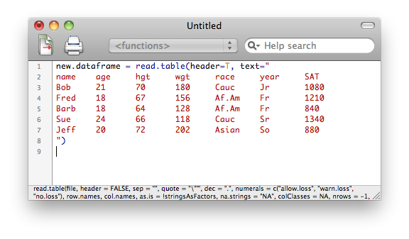
You can save the contents of this window as an R script, which you can always
reopen and modify if necessary.
Further hint: I just got those data into R by copying and pasting the
command and data above directly into the R Console. So that worked. It led
me to wonder if I could copy and paste an HTML table-formatted object from a
web page. I just tried it, and it caused R to crash, so I can't recommend it!
(That's only the second time in 12 years that R has crashed on me.)
However, here's what did work. I copied the contents of the table on the
web page and pasted it into a text editor (I used TextWrangler on a Mac). Then
I added the necessary R commands in the text editor and copied and pasted it
into the R Console. Sure beats typing in that data myself!
Subsetting a Data Frame (optional)
We will use a data frame called USArrests for this exercise.
> data(USArrests)
> head(USArrests)
           Murder Assault UrbanPop Rape
Alabama      13.2     236       58 21.2
Alaska       10.0     263       48 44.5
Arizona       8.1     294       80 31.0
Arkansas      8.8     190       50 19.5
California    9.0     276       91 40.6
Colorado      7.9     204       78 38.7
Here is another useful function for looking at a data frame. The head() function shows the first six lines of data
(cases) inside a data frame. There is also a tail() function that shows the last six lines, and
the number of lines shown can be changed with an option (see the help
pages).
In this case we have a data frame with row names set to state names and
containing variables that give the crime rates (per 100,000 population) for
Murder, Assault, and Rape, as well as the percentage of the population that
lives in urban areas. These data are from 1973 so are not current.
Because state names are used as row names, to see the data for any state,
all we have to do is be able to spell the name of the state.
> USArrests["Pennsylvania",]           # No column index, so all columns displayed.
             Murder Assault UrbanPop Rape
Pennsylvania    6.3     106       72 14.9
We do not have to figure out what the index number would be for that row.
Thus, explicit row names can be very handy. To display the entire row of data
for PA, we just leave out the column index, but THE COMMA STILL HAS TO BE
THERE! Otherwise, you are trying to index a two-dimensional data object using
only one index, and R will tell you to knock it off!
Let's answer the following questions from these data.
- Which state has the lowest murder rate?
- Which states have murder rates less than 4.0?
- Which states are in the top quartile for urban population?
> min(USArrests$Murder)                     # What is the minimum murder rate?
[1] 0.8
> which(USArrests$Murder == 0.8)            # Which line of the data is that?
[1] 34
> USArrests[34,]                            # Give me the data from that line.
             Murder Assault UrbanPop Rape
North Dakota    0.8      45       44  7.3
> USArrests[USArrests$Murder==min(USArrests$Murder),]      # All at once (showing off).
             Murder Assault UrbanPop Rape
North Dakota    0.8      45       44  7.3
>
> which(USArrests$Murder < 4.0)                  # Gives the result in a vector.
 [1]  7 12 15 19 23 29 34 39 41 44 45 49
> USArrests[which(USArrests$Murder < 4.0),]      # Use that vector as an index.
              Murder Assault UrbanPop Rape
Connecticut      3.3     110       77 11.1
Idaho            2.6     120       54 14.2
Iowa             2.2      56       57 11.3
Maine            2.1      83       51  7.8
Minnesota        2.7      72       66 14.9
New Hampshire    2.1      57       56  9.5
North Dakota     0.8      45       44  7.3
Rhode Island     3.4     174       87  8.3
South Dakota     3.8      86       45 12.8
Utah             3.2     120       80 22.9
Vermont          2.2      48       32 11.2
Wisconsin        2.6      53       66 10.8
>
> summary(USArrests$UrbanPop)
   Min. 1st Qu.  Median    Mean 3rd Qu.    Max.
  32.00   54.50   66.00   65.54   77.75   91.00
> USArrests[which(USArrests$UrbanPop >= 77.75),]
              Murder Assault UrbanPop Rape
Arizona          8.1     294       80 31.0
California       9.0     276       91 40.6
Colorado         7.9     204       78 38.7
Florida         15.4     335       80 31.9
Hawaii           5.3      46       83 20.2
Illinois        10.4     249       83 24.0
Massachusetts    4.4     149       85 16.3
Nevada          12.2     252       81 46.0
New Jersey       7.4     159       89 18.8
New York        11.1     254       86 26.1
Rhode Island     3.4     174       87  8.3
Texas           12.7     201       80 25.5
Utah             3.2     120       80 22.9
Suppose we wanted to work with data only from these states. How can we
extract them from the data frame and make a new data frame that contains only
those states? I'm glad you asked.
> subset(USArrests, subset=(UrbanPop >= 77.75)) -> high.urban
> high.urban
              Murder Assault UrbanPop Rape
Arizona          8.1     294       80 31.0
California       9.0     276       91 40.6
Colorado         7.9     204       78 38.7
Florida         15.4     335       80 31.9
Hawaii           5.3      46       83 20.2
Illinois        10.4     249       83 24.0
Massachusetts    4.4     149       85 16.3
Nevada          12.2     252       81 46.0
New Jersey       7.4     159       89 18.8
New York        11.1     254       86 26.1
Rhode Island     3.4     174       87  8.3
Texas           12.7     201       80 25.5
Utah             3.2     120       80 22.9
The subset() function does the trick. The
syntax is a little squirrelly, so let me go through it. The first thing you
give is the name of the data frame. That is followed by the subset= option.
Then inside of parentheses (which actually aren't necessary) give the test
that defines the subset. Store the output into a new data object so that you
can then work with it. Functions that take a data= option can also take a
subset option, so it's a useful thing to know.
Of course you can also use subset()
without an assignment if you just want to display the results. This
eliminates the need to do the fancy indexing tricks above. Or you can use the
fancy indexing tricks with an assignment to get the same result stored in a
new data object. Whatever paddles your canoe. In R there are generally multiple
ways to accomplish things, and this is a good example.
You can clean up your workspace now, but KEEP anorexia and my.data.
Stacking and Unstacking (optional)
Suppose someone has retained your services as a data analyst and gives you
his data (from an Excel file or something) in this format.
contr     treat1    treat2
---------------------------
  22        32        30
  18        35        28
  25        30        25
  25        42        22
  20        31        33
---------------------------
If you're working for free, you can yell at him and make him do it the right
way, but if you're being paid, you probably shouldn't. Here's how to
deal with it. First, let's get these data into a "data frame" in this format,
and I will leave out the command prompts so that you can just copy and paste
these three lines directly into R.
### start copying here
wrong.data = data.frame(contr = c(22,18,25,25,20),
                        treat1 = c(32,35,30,42,31),
                        treat2 = c(30,28,25,22,33))
### stop copying here and paste into R

> wrong.data
  contr treat1 treat2
1    22     32     30
2    18     35     28
3    25     30     25
4    25     42     22
5    20     31     33
Now do this.
> stack(wrong.data) -> correct.data
> correct.data
   values    ind
1      22  contr
2      18  contr
3      25  contr
4      25  contr
5      20  contr
6      32 treat1
7      35 treat1
8      30 treat1
9      42 treat1
10     31 treat1
11     30 treat2
12     28 treat2
13     25 treat2
14     22 treat2
15     33 treat2

> colnames(correct.data) = c("scores","groups")
> head(correct.data)
  scores groups
1     22  contr
2     18  contr
3     25  contr
4     25  contr
5     20  contr
6     32 treat1
And there you go. Now you have a proper data frame.
There is also an unstack() function that
does the reverse of this, and it will work automatically on a data frame that
has been created by stack(), but otherwise is
a little trickier to use. You probably won't have to use it much, so I'll
refer you to the help page if you ever need it (and good luck to you!).
You can remove these data objects. We won't use them again.
Going From Wide to Long and Long to Wide (eventually you'll probably need to know this)
I mentioned this above under "An Ambiguous Case." There are two kinds of data
frames in R, and in most statistical software: wide ones and long ones. If you
deleted the "anorexia" data frame from your workspace, it's easy enough to get
back. Here's how to fetch
the "anorexia" data again (and we'll do it without attaching the MASS
package this time).
> data(anorexia, package="MASS")
What we are about to do is a little confusing until you get some experience
with it, so it will be necessary to be able to see what's happening. The
anorexia data frame is too long to print to a single console screen without
causing it to scroll, so I'm going to cut it down to only nine cases, three
from each group. This will help us to see the difference between wide and long
data frames without constantly scrolling the console window.
> anor = anorexia[c(1,2,3,27,28,29,56,57,58),]
> anor
   Treat Prewt Postwt
1   Cont  80.7   80.2
2   Cont  89.4   80.1
3   Cont  91.8   86.4
27   CBT  80.5   82.2
28   CBT  84.9   85.6
29   CBT  81.5   81.4
56    FT  83.8   95.2
57    FT  83.3   94.3
58    FT  86.0   91.5
I also shortened up the name of our data frame, because we're going to be
typing it a lot.
This is a wide data frame (wide format). It's wide because each line of
the data frame
contains information on ONE SUBJECT, even though that subject was measured
multiple times (twice) on weight (Prewt, Postwt). So all the data for each
subject goes on ONE LINE, even though we could interpret this as a repeated
measures design, or longitudinal data.
In a long format data frame, each value of weight (if we consider that as a
single variable) would define a case. So each of
these subjects would have two lines in such a data frame, one for the subject's
Prewt, and one for her Postwt. A wide data frame would be used, for example, in
analysis of covariance. A long data frame would be used in repeated measures
analysis of variance. Do we have to retype the data frame to get from wide to
long? Fortunately not! Because R has a function called reshape() that will do the work for us.
It is not an easy function to understand, however (and don't count on the
help page being a whole lot of help!). So let me illustrate it, and then I will
explain what's happening.
> reshape(data=anor, direction="long",
+         varying=c("Prewt","Postwt"), v.names="Weight",
+         idvar="subject", ids=row.names(anor),
+         timevar="PrePost", times=c("Prewt","Postwt")
+        ) -> anor.long
> anor.long
          Treat PrePost Weight subject
1.Prewt    Cont   Prewt   80.7       1
2.Prewt    Cont   Prewt   89.4       2
3.Prewt    Cont   Prewt   91.8       3
27.Prewt    CBT   Prewt   80.5      27
28.Prewt    CBT   Prewt   84.9      28
29.Prewt    CBT   Prewt   81.5      29
56.Prewt     FT   Prewt   83.8      56
57.Prewt     FT   Prewt   83.3      57
58.Prewt     FT   Prewt   86.0      58
1.Postwt   Cont  Postwt   80.2       1
2.Postwt   Cont  Postwt   80.1       2
3.Postwt   Cont  Postwt   86.4       3
27.Postwt   CBT  Postwt   82.2      27
28.Postwt   CBT  Postwt   85.6      28
29.Postwt   CBT  Postwt   81.4      29
56.Postwt    FT  Postwt   95.2      56
57.Postwt    FT  Postwt   94.3      57
58.Postwt    FT  Postwt   91.5      58
In this example, the first argument I gave to the
reshape() function was the name of the data frame to be reshaped,
and that was given in the data= argument. Then I specified the direction=
argument as "long" so that the data frame would be converted TO a long
format.
In the second line of this command, I specified varying= as a vector of
variable names in anor that correspond to the repeated measures or longitudinal
measures (the time-varying variables). These values will be given in one column
in the new data frame, so I named that new column using the v.names= argument.
A long data frame needs two things that a wide one does not have. One of
those things is a column identifying the subject (case or experimental unit)
from which the data in a row of the data frame come from. This is necessary
because each subject will have multiple rows of data in a long data frame. So
I used the idvar= argument to specify the name of this new column that would
identify the subjects. I then used ids= to specify how the subjects were to
be named. I told it to use the row names from anor, which is a sensible thing
to do.
The other thing a long format data frame needs that a wide one does not is
a variable giving the condition (or time) in which the subject is being
measured for this particular row of data. In the wide format, this information
is in the column (variable) names, but that will no longer be true in the long
format. We need to know which measure is Prewt and which measure is Postwt for
each subject, since these will be on different rows of the data frame in long
format. I named this new variable using the timevar= argument, and I gave its
possible values in a vector using the times= argument. The order in which those
values should be listed is the same as the order in which the corresponding
columns occur in the wide data frame.
Finally, I closed the parentheses on the
reshape() function and assigned the output to a new data object.
Done! Whew!
This can also be made to work if you have more than one repeated measures
variable, in which case all I can say is may the saints be with you! Surely
there must be an easier syntax for this!!
If the data frame results from a
reshape() command, then it can be converted back very simply.
All you have to do is this.
> reshape(anor.long)
         Treat subject Prewt Postwt
1.Prewt   Cont       1  80.7   80.2
2.Prewt   Cont       2  89.4   80.1
3.Prewt   Cont       3  91.8   86.4
27.Prewt   CBT      27  80.5   82.2
28.Prewt   CBT      28  84.9   85.6
29.Prewt   CBT      29  81.5   81.4
56.Prewt    FT      56  83.8   95.2
57.Prewt    FT      57  83.3   94.3
58.Prewt    FT      58  86.0   91.5
The row names have gone a little screwy, but all the correct information is
there. This isn't very useful actually, because we already have the data in
wide format in the data frame anor, which we were smart enough not to
overwrite. So let's see how to convert from long to wide the hard way.
First, we will get rid of those ridiculous row names.
> rownames(anor.long) <- as.character(1:18)      # Just do it!
> anor.long
   Treat PrePost Weight subject
1   Cont   Prewt   80.7       1
2   Cont   Prewt   89.4       2
3   Cont   Prewt   91.8       3
4    CBT   Prewt   80.5      27
5    CBT   Prewt   84.9      28
6    CBT   Prewt   81.5      29
7     FT   Prewt   83.8      56
8     FT   Prewt   83.3      57
9     FT   Prewt   86.0      58
10  Cont  Postwt   80.2       1
11  Cont  Postwt   80.1       2
12  Cont  Postwt   86.4       3
13   CBT  Postwt   82.2      27
14   CBT  Postwt   85.6      28
15   CBT  Postwt   81.4      29
16    FT  Postwt   95.2      56
17    FT  Postwt   94.3      57
18    FT  Postwt   91.5      58
And now for the reshaping. I won't bother storing it.
> reshape(data=anor.long, direction="wide",
+         v.names=c("Weight"),
+         idvar="subject",
+         timevar="PrePost"
+        )
  Treat subject Weight.Prewt Weight.Postwt
1  Cont       1         80.7          80.2
2  Cont       2         89.4          80.1
3  Cont       3         91.8          86.4
4   CBT      27         80.5          82.2
5   CBT      28         84.9          85.6
6   CBT      29         81.5          81.4
7    FT      56         83.8          95.2
8    FT      57         83.3          94.3
9    FT      58         86.0          91.5
We didn't quite recover the original table, but then we probably didn't really
want to. The first two arguments name the data frame we are reshaping and tell
the direction we are reshaping TO. The next argument, v.names=, gives the name of
the time-varying variable that will be split into two (or more) columns. The
idvar= argument gives the name of the variable that is the subject identifier.
Finally, the timevar= argument gives the name of the variable that contains the
conditions under which the longitidinal information was collected; i.e., there
were two weights, a Prewt and a Postwt. Notice these values were used to name
the two new columns of Weight data. Want a pneumonic to help you remember all
that? Yeah, me too!
Clean up. Get rid of everything EXCEPT my.data.
Working With Spreadsheets and CSV Files (optional)
Even if you can get the spreadsheet-like data editing interface in R to
work for you, it's still really no great shakes. Even when I'm in Windows
(where it works), I use a spreadsheet to manage my data files, especially
larger ones. I'm going to type the data in my.data into a spreadsheet. I use
OpenOffice Calc. You can use whatever.
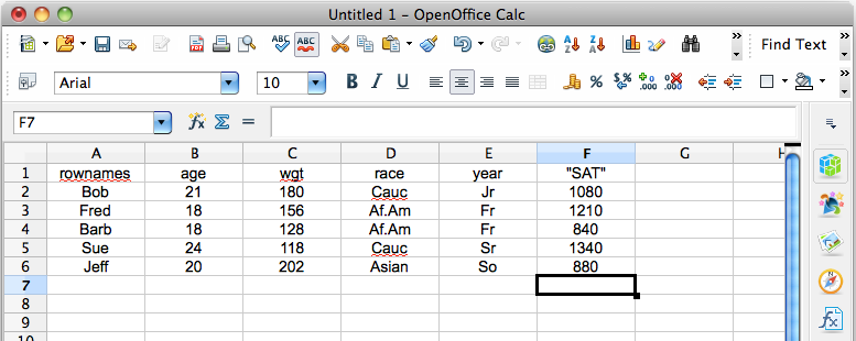
At this point, I can copy and paste any one of those columns into scan(). That's handy, but it's not why I created the
spreadsheet. (Notice that Calc wouldn't let me type SAT into a column header.
It kept insisting it was Sat, abbreviation for Saturday. I HATE software that
thinks it knows what I want! That's why I don't use Excel, but the open source
spreadsheets are getting just as bad. Don't presume you know what I want. JUST
DO WHAT I'M TELLING YOU!!! Gasp! I am so sick and tired of software--and
operating systems--being written for morons! My computer is not a phone, it's
not an iPad, it's a computer. Stop turning it into a toy! And if I want SAT to
be Sat, I'll damn well type it that way! There! That will do
no good whatsoever, but at least I vented.)
Now I'm going to save that as a CSV file. (And once again, my computer will
nag the crap out of me--in Excel especially. "Are you really sure you want to
do this? You're going to lose your formatting." Just do what I tell
you to do and SHUT UP! Anyone who doesn't know what a CSV file is and that it
contains no formatting can use a damn typewriter!) To do that I pulled down the
File menu (you're on your own with that idiot ribbon bar in Excel!), I chose
Save As..., and in the dialog box I entered mydata.csv as the file name, I
specified where to save (Desktop--I'll deal with it from there), and I chose
File type: Text CSV. I chose to edit the filter settings because who knows
how they might have them set? Then I clicked Save. Then it nagged me, and I
clicked Keep Current Format (because there was no choice that said Do What I
Tell You--I'm The Human Here!). In the filter settings I made sure the Field
delimiter was set to a comma (which is what it should always be because, hey,
CSV means comma separated values), and I removed the Text delimiter. Then I
clicked OK. Then I clicked away another warning popup. (See how hard they make
this because every idiot has to be able to use a computer these days?)
Here's what the CSV file actually looks like, and if you don't want to have
to deal with a nagging spreadsheet, you can just type this into a plain text
editor. You can even save it with a .txt extension. R won't care. ("THANK YOU"
to the people who write the R software for not treating me like I'm
feebleminded!)
rownames,age,wgt,race,year,"SAT"
Bob,21,180,Cauc,Jr,1080
Fred,18,156,Af.Am,Fr,1210
Barb,18,128,Af.Am,Fr,840
Sue,24,118,Cauc,Sr,1340
Jeff,20,202,Asian,So,880
Drop this file into your working directory (Rspace), and then read it into R
like this.
> my.newdata = read.csv(file="mydata.csv", row.names="rownames")
> # notice there is no annoying message telling you this has been done!
> my.newdata
     age wgt  race year  SAT
Bob   21 180  Cauc   Jr 1080
Fred  18 156 Af.Am   Fr 1210
Barb  18 128 Af.Am   Fr  840
Sue   24 118  Cauc   Sr 1340
Jeff  20 202 Asian   So  880
Yay! R even dealt with those annoying quotes around SAT. Since "rownames" was
the first column in the file, you could also have set that option as row.names=1. Now suppose somehow your CSV file gets some
whitespace in it. This could happen due to mistyping in the spreadsheet, or
because you typed it that way intentionally into a text editor. (It would be
easier in that case just to leave out the commas and use read.table). (NOTE:
SPSS data files tend to have variable names and value labels padded with white
space, an idiot programming practice if ever there was one!) Do this.
If the file looks something like this...

rownames,  age,  wgt,  race,  year,  SAT
Bob,       21,   180,  Cauc,  Jr,    1080
Fred,      18,   156,  Af.Am, Fr,    1210
Barb,      18,   128,  Af.Am, Fr,    840
Sue,       24,   118,  Cauc,  Sr,    1340
Jeff,      20,   202,  Asian, So,    880

Do this...

> my.newdata = read.csv(file="mydata.csv", row.names=1, strip.white=T)
I personally think using a spreadsheet for a data file this small would be like
driving in a tack with a sledge hammer, but it's up to you. A spreadsheet comes
in very handy for dealing with large data files, however.
Before you quit today, clean everything out of your workspace EXCEPT my.data,
then save the workspace when you quit.
revised 2016 January 21
| Table of Contents
| Function Reference
| Function Finder
| R Project |
|