
| Table of Contents
| Function Reference
| Function Finder
| R Project |
BLOCKING, SPLIT PLOTS, AND LATIN SQUARES
Block Designs
Recall the Related Measures t-Test tutorial,
in which we looked at this example.
schizophrenia = read.table(header=T, text="
pair   affected   unaffected
1      1.27       1.94
2      1.63       1.44
3      1.47       1.56
4      1.39       1.58
5      1.93       2.06
6      1.26       1.66
7      1.71       1.75
8      1.67       1.77
9      1.28       1.78
10     1.85       1.92
11     1.02       1.25
12     1.34       1.93
13     2.02       2.04
14     1.59       1.62
15     1.97       2.08
")
The data are from monozygotic twins discordant for schizophrenia, and the
response measure is left hippocampal size in cubic centimeters. The "pairs" are
the twin pairs. Here we considered monozygosity to be a matching variable. We
could just as easily, and correctly, have called it a blocking variable.
Recall the Single Factor Repeated Measures
tutorial, in which we looked at this example.
groceries = read.table(header=T, row.names=1, text="
subject            storeA  storeB  storeC  storeD
lettuce              1.17    1.78    1.29    1.29
potatoes             1.77    1.98    1.99    1.99
milk                 1.49    1.69    1.79    1.59
eggs                 0.65    0.99    0.69    1.09
bread                1.58    1.70    1.89    1.89
cereal               3.13    3.15    2.99    3.09
ground.beef          2.09    1.88    2.09    2.49
tomato.soup          0.62    0.65    0.65    0.69
laundry.detergent    5.89    5.99    5.99    6.99
aspirin              4.46    4.84    4.99    5.15
")
The data are from four grocery stores near my home, and the response is price of
a grocery item in dollars. I called this a repeated measures design in that
tutorial, but it might more correctly be called a matched groups design. I called
the grocery items subjects, but they might (would!) more appropriately be called
blocks. The analysis would be the same no matter how we fiddle with the
vocabulary.
To refresh your memory, the analysis was done this way.
> groc = stack(groceries)              # we need a data frame in long format
> head(groc)
  values    ind
1   1.17 storeA
2   1.77 storeA
3   1.49 storeA
4   0.65 storeA
5   1.58 storeA
6   3.13 storeA
> colnames(groc) = c("price","store")
> groc$block = rep(rownames(groceries), times=4)      # we need a blocks identifier...
> groc$block = factor(groc$block)                     # which is declared a factor
> head(groc)
  price  store    block
1  1.17 storeA  lettuce
2  1.77 storeA potatoes
3  1.49 storeA     milk
4  0.65 storeA     eggs
5  1.58 storeA    bread
6  3.13 storeA   cereal
> ### question: why can't we use grocery items as row names anymore? ###
> aov.out = aov(price ~ store + Error(block/store), data=groc)  # store within blocks
> summary(aov.out)

Error: block
          Df Sum Sq Mean Sq F value Pr(>F)
Residuals  9  115.2    12.8

Error: block:store
          Df Sum Sq Mean Sq F value Pr(>F)
store      3 0.5859 0.19529   4.344 0.0127 *
Residuals 27 1.2137 0.04495
---
Signif. codes:  0 '***' 0.001 '**' 0.01 '*' 0.05 '.' 0.1 ' ' 1
Similarly, we could do it this way.
> aov.out = aov(price ~ block + store, data=groc)    # treatment by blocks approach
> summary(aov.out)
            Df Sum Sq Mean Sq F value Pr(>F)
block        9 115.19  12.799 284.722 <2e-16 ***
store        3   0.59   0.195   4.344 0.0127 *
Residuals   27   1.21   0.045
---
Signif. codes:  0 '***' 0.001 '**' 0.01 '*' 0.05 '.' 0.1 ' ' 1
In the same tutorial, we considered the following example, which is a true
repeated measures design.
EMG = read.table(header=T, text="
subj LB1 LB2 LB3  LB4
S1   143 368 345  772
S2   142 155 161  178
S3   109 167 356  956
S4   123 135 137  187
S5   276 216 232  307
S6   235 386 398  425
S7   208 175 207  293
S8   267 358 698  771
S9   183 193 631  403
S10  245 268 572 1383
S11  324 507 556  504
S12  148 378 342  796
S13  130 142 150  173
S14  119 171 333 1062
S15  102  94  93   69
S16  279 204 229  299
S17  244 365 392  406
S18  196 168 199  287
S19  279 358 822  671
S20  167 183 731  203
S21  345 238 572 1652
S22  524 507 520  504
")
The data are EMG amplitudes from the left forehead of 22 subjects under
different conditions of emotional arousal. Our subj(ects) column could just as
easily be called blocks, and the analysis would once again be the same. In a
repeated measures (or within subjects) design, the subjects are the blocking
variable.
In a treatment by blocks design we have subjects (experimental units)
matched on some blocking variable that makes them somehow similar to one
another in a way that should influence their response to the experimental
treatments. In other words, a treatment by blocks design is what we would call
a matched groups design when there are two levels of treatment and we are
contemplating a t-test, except there are more than two levels of the treatment,
and we are therefore contemplating an ANOVA.
Once the subjects are matched (blocked), if they are then randomly assigned
to treatment conditions within blocks--which is not true in any of the above
examples--then we have a randomized blocks design. If every block has a subject
in every condition, then it's a randomized complete blocks design. If that's
not the case, then it's a randomized incomplete blocks design.
An important assumption of treatment by blocks designs is that there is no
treatment-by-blocks interaction in the population. Any interaction-like
variability in the sample is assumed to be random error and constitutes the
error term for the ANOVA. Unless...
Replication
What if there is replication (more than one subject) in each of the
treatment-by-blocks design cells? This wouldn't happen in a repeated measures
design where subjects ARE the blocks, but it could easily happen in a treatment
by blocks design where the blocks are something other than subjects. Myers
(1972) gives the following exercise in his textbook.
| | A1 | A2 | A3 |
| block 1 | 1, 2 | 16, 10 | 3, 1 |
| block 2 | 4, 3 | 13, 12 | 3, 3 |
| block 3 | 6, 8 | 7, 10 | 9, 5 |
| block 4 | 10, 8 | 7, 7 | 5, 12 |
Data entry is straightforward. (I've always wanted to say something like that!)
### in a script window I typed...
Myers = read.table(header=T, text="
block  treat  score
B1     A1     1
B1     A1     2
B1     A2     16
B1     A2     10
B1     A3     3
B1     A3     1
B2     A1     4
B2     A1     3
B2     A2     13
B2     A2     12
B2     A3     3
B2     A3     3
B3     A1     6
B3     A1     8
B3     A2     7
B3     A2     10
B3     A3     9
B3     A3     5
B4     A1     10
B4     A1     8
B4     A2     7
B4     A2     7
B4     A3     5
B4     A3     12
")
### if you copy to here, you can paste it into the R Console

>summary(Myers)
 block  treat      score
 B1:6   A1:8   Min.   : 1.000
 B2:6   A2:8   1st Qu.: 3.000
 B3:6   A3:8   Median : 7.000
 B4:6          Mean   : 6.875
               3rd Qu.:10.000
               Max.   :16.000
The trick to getting the analysis right is having R recognize the correct
error term. Myers shows that the correct error term is subject variability
within block-by-treatment cells. But hold on just a second! Isn't that the same
error term we would use if we merely analyzed this as a two-factor factorial
design? Yes, it is. Which raises an interesting question. (Okay, it's
interesting to me!)
Suppose we have a two-factor design in which one of our factors is a true
experimental variable (i.e., we can randomly assign subjects to its levels),
but the other factor is quasi-experimental (consists of intact groups). Let's
say the quasi-experimental factor is gender. Then don't we have a restriction
on randomization? Subject Sally cannot be assigned to the level of gender we
would call males, and subject Fred can only be assigned to that level. Doesn't
that make gender a blocking variable? Yes it does, but it doesn't matter
whether we consider it a blocking variable or a second IV. When we have
replication in the cells, the analysis is the same. I suppose we'd be inclined
to see it more as a blocking variable if we were not interested in the gender
main effect, but only interested in partialling out the variability due to
gender to get a more sensitive test on our variable of interest. If we're
interested in both the gender main effect and the main effect of the
experimental factor, then gender is a second IV.
So the correct analysis is:
> aov.out = aov(score ~ block * treat, data=Myers)
> summary(aov.out)
            Df Sum Sq Mean Sq F value   Pr(>F)
block        3  25.46    8.49   1.629 0.234657
treat        2 136.75   68.37  13.128 0.000953 ***
block:treat  6 153.92   25.65   4.925 0.009218 **
Residuals   12  62.50    5.21
---
Signif. codes:  0 '***' 0.001 '**' 0.01 '*' 0.05 '.' 0.1 ' ' 1
I am gratified to see that this is the answer "in the back of the book!"
Myers further points out that the larger the mean square is for block and
block:treat, the more efficient the block design should be over the
corresponding single factor design in which only treat is tested. In other
words, if gender is unrelated to variability in the DV, then DON'T include it
as a blocking variable. It will just end up costing you degrees of freedom
in the error term. (For the record, the one-way ANOVA result is F(2,21) =
5.936, p = .009.)
- Myers, J. L. (1972). Fundamentals of Experimental Design. Boston: Allyn
and Bacon.
Split Plot Designs
A split plot design is a block design. Suppose we wish to test five varieties
of seed to see how successfully we can grow corn from them. We have a large
field in which to do the tests. The field is somewhat heterogeneous in its
characteristics, however, so we decide to divide the field into plots with
more uniform characteristics. Then each plot is split into five gardens, and
one variety of seed is assigned at random to each garden within each plot.
This is a randomized complete blocks design. It is analyzed just as any other
treatment by blocks design would be (above).
Split plot designs get interesting when we further subdivide our plots.
Suppose we have several fields in which to do the tests. We divide each field
into homogeneous plots, and each plot into five gardens, etc. Now we have
gardens within plots within fields.
A source that is rife with such agricultural examples is Crawley (2005).
We have to go to his website to download his data sets. They will download
as a file called zipped.zip. Unzip it, rename the folder "Crawley", and drop it
into your normal working directory (Rspace). Then retrieve a data file called
"splityield" as follows.
> yields = read.table(file="Crawley/splityield.csv", header=T, sep=",")
> summary(yields)
     yield        block      irrigation   density   fertilizer
 Min.   : 60.00   A:18   control  :36   high  :24   N :24
 1st Qu.: 86.00   B:18   irrigated:36   low   :24   NP:24
 Median : 95.00   C:18                  medium:24   P :24
 Mean   : 99.72   D:18
 3rd Qu.:114.00
 Max.   :136.00
The experiment was this. Crop yield was measured in response to three factors,
which were irrigation (control, irrigated), sowing density (high, low, medium;
which could be releveled if we were of a mind to), and fertilizer application
(N, NP, and P). Four fields were used, each of which was split in half and a
level of irrigation applied at random to each half. Each half field was split
into three parts and a level of density randomly assigned to each one. Finally,
each of these subsubfields was split again into three parts and a level of
fertilizer assigned at random to each one. Thus, we have fertilizer within
density within irrigation, and the whole thing within fields or blocks.
Crawley suggests the following analysis.
> aov.out = aov(yield ~ irrigation * density * fertilizer +
+               Error(block/irrigation/density/fertilizer), data=yields)
> summary(aov.out)

Error: block
          Df Sum Sq Mean Sq F value Pr(>F)
Residuals  3  194.4   64.81

Error: block:irrigation
           Df Sum Sq Mean Sq F value Pr(>F)
irrigation  1   8278    8278   17.59 0.0247 *
Residuals   3   1412     471
---
Signif. codes:  0 '***' 0.001 '**' 0.01 '*' 0.05 '.' 0.1 ' ' 1

Error: block:irrigation:density
                   Df Sum Sq Mean Sq F value Pr(>F)
density             2   1758   879.2   3.784 0.0532 .
irrigation:density  2   2747  1373.5   5.912 0.0163 *
Residuals          12   2788   232.3
---
Signif. codes:  0 '***' 0.001 '**' 0.01 '*' 0.05 '.' 0.1 ' ' 1

Error: block:irrigation:density:fertilizer
                              Df Sum Sq Mean Sq F value   Pr(>F)
fertilizer                     2 1977.4   988.7  11.449 0.000142 ***
irrigation:fertilizer          2  953.4   476.7   5.520 0.008108 **
density:fertilizer             4  304.9    76.2   0.883 0.484053
irrigation:density:fertilizer  4  234.7    58.7   0.680 0.610667
Residuals                     36 3108.8    86.4
---
Signif. codes:  0 '***' 0.001 '**' 0.01 '*' 0.05 '.' 0.1 ' ' 1
Subsequent analysis is suggested by Crawley in his textbook. (Note: The
smallest level of subdivision does not need to be included in the Error term,
so in his textbook Crawley gives Error(block/irrigation/density), which is
equivalent. Similarly, in the groceries example of the last section, we could
have given Error(blocks) as the error term.)
Latin Square Designs
A Latin square design is a block design. Suppose you have a treatment of
interest that has three levels. You decide to divide your subjects into three
blocks to partial out variability due to a certain nuisance variable. Then you
think of a second nuisance variable, and you decide to block on that variable
as well (also three blocks). Now you've got a 3x3x3 factorial design, for a
total of 27 cells in the design table. Problem is, you don't have that many
subjects (experimental units) available.
Latin square is a possible solution. Let's draw the design table for the
two blocking factors, which we'll call M and N.
Your treatment has three levels, which we'll call A, B, and C. The trick is to
assort those treatment levels to the cells in such a way that no treatment level
occurs more than once in each row and each column. That's a Latin square.
There are several possible rearrangements of this particular square, which can
be obtained by permuting the rows and columns. One of those should be chosen
at random.
We no longer have a full factorial design with 3x3x3=27 design cells. We
now have a 3x3 Latin square, and at one subject per cell, we need only 9 total
subjects (experimental units). We will not be able to analyze interactions in
such a design (see below), so we have to assume they don't exist. Any
interaction-like variability will be assumed to be nothing more than random
noise and will constitute the error term.
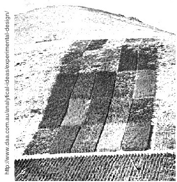
An agricultural experiment with a Latin square structure.
The built-in data set OrchardSprays illustrates an 8x8 Latin square design.
Here is the description from the help page.
     An experiment was conducted to assess the potency of various constituents
     of orchard sprays in repelling honeybees, using a Latin square design.
     Individual cells of dry comb were filled with measured amounts of lime
     sulphur emulsion in sucrose solution. Seven different concentrations of
     lime sulphur ranging from a concentration of 1/100 to 1/1,562,500 in
     successive factors of 1/5 were used as well as a solution containing no
     lime sulphur.

     The responses for the different solutions were obtained by releasing 100
     bees into the chamber for two hours, and then measuring the decrease in
     volume of the solutions in the various cells.

     An 8 x 8 Latin square design was used and the treatments were coded as follows:
     A  highest level of lime sulphur
     B  next highest level of lime sulphur
     ...
     G  lowest level of lime sulphur
     H  no lime sulphur
I'm not sure exactly why you'd want to repel honeybees from your orchard, but
then I'm not an agronomist, so let's just look at the data.
> data(OrchardSprays)
> OS = OrchardSprays              # I'm not typing OrchardSprays any more than necessary!
> summary(OS)
    decrease          rowpos         colpos       treatment
 Min.   :  2.00   Min.   :1.00   Min.   :1.00   A      : 8
 1st Qu.: 12.75   1st Qu.:2.75   1st Qu.:2.75   B      : 8
 Median : 41.00   Median :4.50   Median :4.50   C      : 8
 Mean   : 45.42   Mean   :4.50   Mean   :4.50   D      : 8
 3rd Qu.: 72.00   3rd Qu.:6.25   3rd Qu.:6.25   E      : 8
 Max.   :130.00   Max.   :8.00   Max.   :8.00   F      : 8
                                                (Other):16
> OS$rowpos = factor(OS$rowpos)   # the row ...
> OS$colpos = factor(OS$colpos)   # and column blocking factors must be seen by R as factors!
> with(OS, table(rowpos,colpos))  # an unreplicated Latin square (n=1 per cell)
      colpos
rowpos 1 2 3 4 5 6 7 8
     1 1 1 1 1 1 1 1 1
     2 1 1 1 1 1 1 1 1
     3 1 1 1 1 1 1 1 1
     4 1 1 1 1 1 1 1 1
     5 1 1 1 1 1 1 1 1
     6 1 1 1 1 1 1 1 1
     7 1 1 1 1 1 1 1 1
     8 1 1 1 1 1 1 1 1
> matrix(OS$treatment, nrow=8)    # and here is the Latin square
     [,1] [,2] [,3] [,4] [,5] [,6] [,7] [,8]
[1,] "D"  "C"  "F"  "H"  "E"  "A"  "B"  "G"
[2,] "E"  "B"  "H"  "A"  "D"  "C"  "G"  "F"
[3,] "B"  "H"  "A"  "E"  "G"  "F"  "C"  "D"
[4,] "H"  "D"  "E"  "C"  "A"  "G"  "F"  "B"
[5,] "G"  "E"  "D"  "F"  "C"  "B"  "A"  "H"
[6,] "F"  "A"  "C"  "G"  "B"  "D"  "H"  "E"
[7,] "C"  "F"  "G"  "B"  "H"  "E"  "D"  "A"
[8,] "A"  "G"  "B"  "D"  "F"  "H"  "E"  "C"
That last command worked only because the data frame was constructed in such
an orderly fashion.
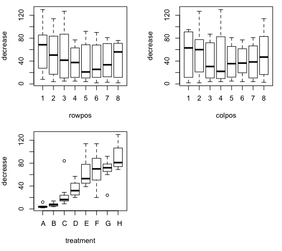
> par(mfrow=c(2,2))
> plot(decrease ~ rowpos + colpos + treatment, data=OS)
Hit <Return> to see next plot:    ### return focus to the Console and press Enter
 The ANOVA is a straightforward additive model.
> aov.out = aov(decrease ~ rowpos + colpos + treatment, data=OS)
> summary(aov.out)
            Df Sum Sq Mean Sq F value   Pr(>F)
rowpos       7   4767     681   1.788    0.115
colpos       7   2807     401   1.053    0.410
treatment    7  56160    8023  21.067 7.45e-12 ***
Residuals   42  15995     381
---
Signif. codes:  0 '***' 0.001 '**' 0.01 '*' 0.05 '.' 0.1 ' ' 1
There is a signicant effect of treatment. A post hoc test could be done with
TukeyHSD(aov.out, which= "treatment"). In this
case, however, a trend analysis might be particularly appropriate. Notice
from the boxplot that there is reason to believe a substantial problem with
heterogeniety of variance exists.
Replicated Latin Square Designs
Now things get messy. There seems to be a difference of opinion among
authorities as to how these designs should be done as well as how they
should be analyzed. Replicated Latin square means you have more than one
subject in each of your design cells. But back the bus up here, because we've
already overlooked our first complication.
Suppose you have four treatments and two four-level blocking factors.
That would require 16 subjects (4 treatment positions times 4 orders). Suppose
you have 32 subjects available.
What are you going to do with the second 16 of them? One possibility would be
to put two subjects in each of your design cells. Thus, you may have choosen
this Latin square:
And in each of those little cells you would have two subjects. That's what
I'm calling "simple replication." The other possibility would be to
choose, from your handbook of experimental designs, a second Latin square
and put the second sixteen subjects in that. Thus, you may have THESE TWO
Latin squares, which I'll call "replicates":
And in each of those little cells you would have one subject. Another
complication here is just how the replicates are produced. If the experiment
is done today with 16 subjects, and then tomorrow it's done again, and the next
day it's done again, and so on, with the same Latin square, then you've
essentially added a third blocking factor, replicates, and the data should
be analyzed accordingly. However, it's also possible to have different Latin
squares in your replicates, as was the case immediately above. It doesn't seem
to matter. In either case the analysis would be:
score ~ row + column + replicate + treatment
It can get more complex, however. (Of course it can!) The following examples
were taken from
Dr. Iago Hale's site at the University of New Hampshire. We are testing
gasoline additive in tractors but, not only is it possible for the Latin square
to change from replicate to replicate, it's also possible that we might be using
a new set of tractors and a new bunch of drivers.
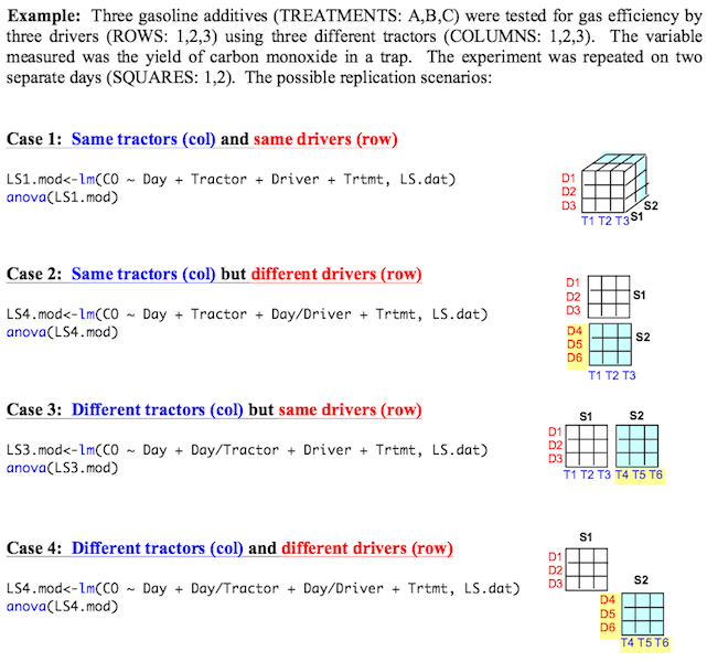
(Note: Dr. Hale uses the lm() function and
anova() extractor function to get the ANOVA instead
of aov() and summary().
The two methods are equivalent.)
I, on the other hand, have not driven a tractor since I was a kid and am
more likely to have a bunch of squirming rats, and I'm just going to stick all
of my cell(3,2) subjects into cell(3,2) and let them squirm around in there.
Thus, I have simple replication but no replicates as such.
Putting the bus in forward gear again, the second issue is whether or not
we should look for interactions in the replicated Latin square. One source I
consulted said, emphatically, NO, that all interactions in Latin square designs
are assumed to be error. Other sources SEEMED to disagree.
In a simple, unreplicated, Latin square, we must ASSUME there are no
interactions, because any variability we see interaction-wise is going to be
treated as noise and dumped into our error term. In fact, we wouldn't have
an error term otherwise. There are not enough degrees of freedom to test an
interaction. But what if those interactions are real, i.e., what if
they exist in nature? In a Latin square design, the treatment effects are
partially confounded with the interactions. Myers (1972) discusses this in
some detail and possible remedies. Bottom line is, the existence of
interactions between the treatment factors and blocking factors is a serious
problem in Latin square designs. An interaction between the blocking factors
(rows x columns) is especially serious, because that interaction is confounded
with the treatment factor.
Latin square designs are often used to control for various kinds of order
effects when there are repeated measures on the treatment of interest. It's
often suggested that this "incomplete counterbalancing" is a good way to
control for effects caused by order of presentation of the treatment levels.
Sometimes it is, sometimes it's not. (I'll cover the analysis of repeated
measures Latin squares in a separate section.)
A number of years ago, a student of ours, Paula Pyle, did her senior research
on aggressive behavior in children resulting from watching violent cartoons.
(The aggressive behaviors, not the children, resulted from watching cartoons.)
She had each child
watch two cartoons, a Power Rangers cartoon (violent) and a Barney cartoon
(nonviolent). After each cartoon, the children engaged in a play session during
which Paula counted the number of aggressive behaviors displayed by the child.
Half of the children saw the Power Rangers cartoon first, and half saw the
Barney cartoon first.
Overall, the children displayed more aggressive behaviors after watching the
Power Rangers cartoon than they did after watching the Barney cartoon. However,
that wasn't the end of the story by a long shot! The children who saw the
Power Rangers cartoon first were more aggressive after seeing the Barney
cartoon than were the children who saw the Barney cartoon first, a clear
carryover effect.
When your subjects are inanimate objects, as they often are in industrial
experiments for example, there are some effects that you probably are not going
to see that may nevertheless occur quite frequently when your subjects are
human beings (or any other sort of experimental unit with a memory). Some of
those "human" effects are going to be seen in interactions.
Example: Suppose seeing the Power Rangers cartoon first causes a carryover
effect resulting in increased aggression after seeing the Barney cartoon, but
seeing the Barney cartoon first does not carry over to the Power Rangers
cartoon. I.e., kids are equally aggressive after the Power Rangers cartoon
regardless of whether they saw it first or second. That's an interaction
between your rows and your columns right there! On the other hand, suppose
seeing Power Rangers first makes kids more aggressive after Barney, and seeing
Barney first makes kids less aggressive after Power Rangers. In fact, suppose
all kids show equal aggression in the two treatments but more aggression
after seeing Power Rangers first than after seeing Barney first. Your overall
treatment effect has just averaged to zero over rows of your design table.
Nevertheless, there is clearly an effect of watching Power Rangers vs. Barney.
Things get complicated when your experimental units have a memory! For
example, a column effect in your Latin square design might be a perfectly
legitimate practice effect, or transfer effect, or fatigue effect. A row
effect might be a very real carryover effect. And if the effect of A carries
over, but the effect of B does not, then you've got a rows by columns
interaction. A Latin square is not always the best design choice.
I suppose the moral of this story should be: THINK FIRST, design later!
Then THINK AGAIN before you analyze!
The problem with the obsessive blocking that occurs in Latin square designs
is that it reduces the degrees of freedom available in the error term. The
following diagram (which I found
at Dr. Hale's site) illustrates this point clearly as you go from completely
randomized (CRD) to randomized complete blocks (RCBD) to Latin square (LS)
designs (assuming 5 treatments and 25 subjects).
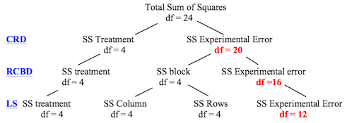
Replication is one way to get more degrees of freedom in your error term.
So back to the case of my squirming rats stuffed into the design cells of my
ONE Latin square, without true time-to-time replicates. This is probably the
case that has occurred most often in psychology. Myers gives an analysis of
such a design when the treatment factor is tested between subjects. Such a
design is not as desirable as the design with true replicates because it is
more prone to interactions (says Myers). The real utility of this design is
as a counterbalancing control for order effects in a repeated measures design,
to which we now move on.
- Myers, J. L. (1972). Fundamentals of Experimental Design. Boston: Allyn
and Bacon.
Latin Square and Repeated Measures: Counterbalancing
A number of years ago, Wes Rowe did, as his senior research project in our
department, an experiment in which he studied the effect of background music on
a card matching task. The subject was seated at a table on which he or she found
an array of cards. The subject's task was to turn over the cards two at a time.
If the cards matched, they were removed from the array. If they did not match,
they were turned face down again, and the subject continued to turn the cards
two at a time. The objective was to match all the cards and remove them from
the array as quickly as possible. Each subject did the task three times, once
with each of three kinds of background music: no music, classical music, and
instrumental rap music.
Thus, we have a repeated measures design. The DV was time to complete the
task (all cards matched and removed from the array), in seconds. I should note
that Wes used complete counterbalancing to control for order effects, which
involved using six orders of treatment, with 8 subjects assigned to each order.
(In effect, that means he had two Latin squares, which could be analyzed as
replicates, with replication within each replicate. We're going to keep things
a little simpler and look at only half of his data.)
I'll give you two options for getting the data. Here is the first. Type the
following with excruciating care!
> file = "http://ww2.coastal.edu/kingw/statistics/R-tutorials/text/rowe.txt"
> match = read.csv(file)
If that didn't work, then you can resort to copying and pasting the following
script.
### begin copying here
match = read.table(header=T, text="
Order Music Time Row Column Subject
CRN    NM  206  R2     C3     S10
CRN    NM  178  R2     C3     S11
CRN    NM  204  R2     C3     S12
CRN    NM  169  R2     C3     S13
CRN    NM  176  R2     C3     S15
CRN    NM  176  R2     C3     S16
CRN    NM  194  R2     C3     S17
CRN    NM  206  R2     C3     S18
NCR    NM  211  R1     C1     S19
NCR    NM  181  R1     C1     S21
NCR    NM  224  R1     C1     S22
NCR    NM  177  R1     C1     S23
NCR    NM  180  R1     C1     S24
NCR    NM  218  R1     C1     S25
NCR    NM  229  R1     C1     S26
NCR    NM  176  R1     C1     S27
RNC    NM  190  R3     C2     S45
RNC    NM  181  R3     C2     S46
RNC    NM  186  R3     C2     S47
RNC    NM  170  R3     C2     S48
RNC    NM  178  R3     C2     S49
RNC    NM  168  R3     C2     S50
RNC    NM  223  R3     C2     S51
RNC    NM  199  R3     C2     S52
CRN    CM  193  R2     C1     S10
CRN    CM  168  R2     C1     S11
CRN    CM  209  R2     C1     S12
CRN    CM  178  R2     C1     S13
CRN    CM  171  R2     C1     S15
CRN    CM  171  R2     C1     S16
CRN    CM  197  R2     C1     S17
CRN    CM  193  R2     C1     S18
NCR    CM  201  R1     C2     S19
NCR    CM  188  R1     C2     S21
NCR    CM  206  R1     C2     S22
NCR    CM  176  R1     C2     S23
NCR    CM  192  R1     C2     S24
NCR    CM  203  R1     C2     S25
NCR    CM  221  R1     C2     S26
NCR    CM  192  R1     C2     S27
RNC    CM  182  R3     C3     S45
RNC    CM  186  R3     C3     S46
RNC    CM  199  R3     C3     S47
RNC    CM  179  R3     C3     S48
RNC    CM  192  R3     C3     S49
RNC    CM  177  R3     C3     S50
RNC    CM  232  R3     C3     S51
RNC    CM  192  R3     C3     S52
CRN   IRM  208  R2     C2     S10
CRN   IRM  163  R2     C2     S11
CRN   IRM  212  R2     C2     S12
CRN   IRM  151  R2     C2     S13
CRN   IRM  168  R2     C2     S15
CRN   IRM  167  R2     C2     S16
CRN   IRM  188  R2     C2     S17
CRN   IRM  185  R2     C2     S18
NCR   IRM  202  R1     C3     S19
NCR   IRM  184  R1     C3     S21
NCR   IRM  200  R1     C3     S22
NCR   IRM  168  R1     C3     S23
NCR   IRM  180  R1     C3     S24
NCR   IRM  161  R1     C3     S25
NCR   IRM  196  R1     C3     S26
NCR   IRM  181  R1     C3     S27
RNC   IRM  166  R3     C1     S45
RNC   IRM  188  R3     C1     S46
RNC   IRM  204  R3     C1     S47
RNC   IRM  177  R3     C1     S48
RNC   IRM  174  R3     C1     S49
RNC   IRM  165  R3     C1     S50
RNC   IRM  226  R3     C1     S51
RNC   IRM  191  R3     C1     S52
")
### end copying here and paste into the R Console
The first thing we should notice is that the Order variable and the Row variable
contain duplicate information, so we can use either one (but not both) in the
analysis. From a summary, then, we can see what Latin square was used.
> summary(match)
 Order    Music         Time       Row     Column     Subject
 CRN:24   CM :24   Min.   :151.0   R1:24   C1:24   S10    : 3
 NCR:24   IRM:24   1st Qu.:176.0   R2:24   C2:24   S11    : 3
 RNC:24   NM :24   Median :187.0   R3:24   C3:24   S12    : 3
                   Mean   :188.9                   S13    : 3
                   3rd Qu.:201.2                   S15    : 3
                   Max.   :232.0                   S16    : 3
                                                   (Other):54
Under the summary for Order we see the Latin square. It says each order was
used 24 times, but that's because we have three lines per subject in the
table (a long format data frame), one for each kind of Music. In fact, there
are only eight Subjects per Order, each subject being used at each of three
levels of Music.
> with(match, table(Order,Music))
     Music
Order CM IRM NM
  CRN  8   8  8
  NCR  8   8  8
  RNC  8   8  8
A quick graphical display of the effects can be had as follows.
> par(mfrow=c(2,2))                                   # partition the graphics device
> plot(Time ~ Order + Column + Music, data=match)     # not boxplot(); I make that mistake often!
Hit <Return> to see next plot:
> with(match, interaction.plot(Column, Order, Time))  # row by column interaction if any
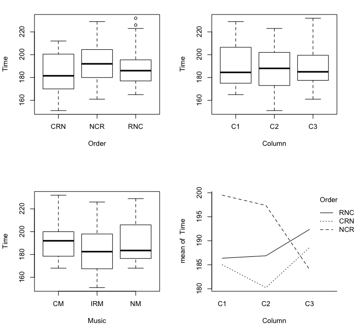 I find that interaction plot disturbing, and disturbing in a disturbingly
meaningful way at that. The longest solving time was in the no music condition
when that condition was done first. If that same effect shows up in the second
Latin square (the advantage of having a replicate!), I'd be quite distressed.
Nevertheless, let's proceed with the analysis to see how it is done (on this
square).
I find that interaction plot disturbing, and disturbing in a disturbingly
meaningful way at that. The longest solving time was in the no music condition
when that condition was done first. If that same effect shows up in the second
Latin square (the advantage of having a replicate!), I'd be quite distressed.
Nevertheless, let's proceed with the analysis to see how it is done (on this
square).
> aov.out = aov(Time ~ Order + Column + Music + Error(Subject/Music), data=match)
> summary(aov.out)

Error: Subject
          Df Sum Sq Mean Sq F value Pr(>F)
Order      2    977   488.7   0.595  0.561
Residuals 21  17252   821.5

Error: Subject:Music
          Df Sum Sq Mean Sq F value  Pr(>F)
Column     2     67    33.5   0.390 0.67935
Music      2   1046   522.8   6.084 0.00465 **
Residuals 44   3781    85.9
---
Signif. codes:  0 '***' 0.001 '**' 0.01 '*' 0.05 '.' 0.1 ' ' 1
We find a significant effect of Music type. Notice that R realized the
Column effect was also within subjects and tested it accordingly. It's
educational to compare this result to the single factor repeated measures
ANOVA and to the mixed factorial ANOVA with Order as a between subjects factor.
I'll leave that to the interested reader.
Here's another interesting (but incorrect) analysis.
> aov.out2 = aov(Time ~ Order * Column + Music + Error(Subject/Music), data=match)
> summary(aov.out2)

Error: Subject
          Df Sum Sq Mean Sq F value Pr(>F)
Order      2    977   488.7   0.595  0.561
Residuals 21  17252   821.5

Error: Subject:Music
             Df Sum Sq Mean Sq F value  Pr(>F)
Column        2     67    33.5   0.426 0.65589
Music         2   1046   522.8   6.645 0.00311 **
Order:Column  2    477   238.4   3.030 0.05897 .
Residuals    42   3304    78.7
---
Signif. codes:  0 '***' 0.001 '**' 0.01 '*' 0.05 '.' 0.1 ' ' 1
The test on Music is the wrong test, as the Order:Column and Residuals (within)
should be combined to do that test. (See the previous table.) However, Myers
pointed out that the test on the Order:Column interaction is interesting as an
indication of whether the row-by-column interaction is large enough to be
distressing, as that is the interaction which is confounded with the treatment
effect. Ideally, that F-ratio should be 1.
created 2016 February 11
| Table of Contents
| Function Reference
| Function Finder
| R Project |
|