You are about to become smarter --or at least better informed statistically-- than the majority of professional psychologists, and probably moreso than most of the psychology professors you'll ever have. In spite of the fact that unbalanced designs have been discussed and debated extensively in psychological journals such as Psychological Review, most psychologists are unfamiliar with the issue.
The reason for this can be stated in four letters: SPSS. The statistical package used most often by psychologists is SPSS. Most psychologists use it without thinking, and so they let SPSS do whatever it wants to do. SPSS (and also SAS and Minitab, the other two major stat packages) does Type III sums of squares for unbalanced designs by default, and most psychologists just let it do so without even realizing what's happening or, for that matter, that the issue even exists.
That's fine IF they are analysing data from a designed (randomized) experiment, but if they are analyzing data from a quasi-experimental design, it may well be the WRONG THING TO DO! Tell you another story. I once had a student in this class (who shall remain unnamed) who went on afterwards to do research with one of our faculty. They were analyzing data from an unbalanced design. The professor used SPSS to do the analysis, while the student used R. They got different answers, and neither of them knew why. The student certainly should have known! SPSS does Type III sums of squares by default, while R does Type I. The student had a chance to show off his statistical sophistication, and he blew it. I should have lowered his grade in the course!!! (Just kidding. I can't do that. Can I?)
Question 1. What is the moral of this story?
Here are the salary data again (from Maxwell and Delany). Fill in the boxes in the cells and then complete the margins. (No Check Answer buttons. Too easy! For those of you who remember the distinction, calculate the marginal means as good old fashioned weighted means, meaning sum in that box divided by n in that box.)
| gender | (row marginals) | |||
| female | male | |||
| education | degree | 24, 26, 25, 24, 27, 24, 27, 23 n = sum = mean = |
25, 29, 27 n = sum = mean = |
n = sum = mean = |
| no.degree | 15, 17, 20, 16 n = sum = mean = |
19, 18, 21, 20, 21, 22, 19 n = sum = mean = |
n = sum = mean = |
|
| (column marginals) | n = sum = mean = |
n = sum = mean = |
N = SUM = MEAN = |
|
Question 2. What did you get for the row marginal means?
Question 3. What effect is shown by these means (if any)? Would you say this
effect exists?
Question 4. What did you get for the column marginal means?
Question 5. What effect is shown by these means (if any)? Would you say this
effect exists?
How did you get the mean in the first column? Did you add the two group sizes to get total n in that column of 12, then add the two group sums to get a total sum in that column of 268, and then divide 268 by 12 to get the column mean? If you did (and that's the way we've learned to do it), then what you've calculated is called a weighted mean. It's called a weighted mean because it can also be calculated this way.
25.0 * 8 + 17.0 * 4   200 + 68
------------------- = -------- = 22.333
      (8 + 4)            12
That is, the group means are multiplied by (weighted by) group sizes, and then added and divided by the sum of the weights. In a weighted mean, the size of the group matters. Larger groups count more (are weighted more heavily) in the calculation of a weighted mean and, therefore, the marginal mean will be closer to the mean of the larger group. The weighted mean is also what you would get if you just forgot there were two groups, added up all the scores in the column, and divided by the number of them. In other words, it's the mean as you've come to know and love it.
There's another way to calculate marginal means, however. Just add the means in that column (or row) and divide by the number of means, as so for the first column.
25.0 + 17.0
----------- = 21.0
     2
In this calculation, the group means are NOT weighted by the group sizes and, therefore, this type of marginal mean is called an unweighted mean (although some people prefer to call them equally weighted means). With unweighted means, all groups count the same regardless of how large the groups are. If the design is balanced, the weighted and unweighted marginal means will be the same. If the design is unbalanced, they probably will not be.
Here's an extreme example from a Psyc 497 project (Zach Rizutto, Spring 2013). M1 = 23.322, n1 = 59, M2 = 28.000, n2 = 1. Calculate the weighted and unweighted means. Here are those calculations. (You'll learn nothing by gawking at them. Get out your calculator!)
23.322 * 59 + 28.000 * 1
------------------------ = 23.400 (weighted mean)
        (59 + 1)

23.322 + 28.000
--------------- = 25.611 (unweighted mean)
       2
This example is not extreme because the two means came out to be extremely different. They didn't, although that can certainly happen. This example is extreme because of the extremely disparate group sizes. In the weighted mean, M1 counts 59 times as much as M2, but every subject counts the same. In the unweighted mean, M1 and M2 count the same, but that 1 subject in group 2 carries the same weight as the 59 subjects in group 1. So as the graphic on the title page of the lecture asked: when does a mouse weigh more than an elephant? It might if you're using unweighted means.
Does that sound fair? Fair doesn't enter into it. The question is, which mean is the correct one? And that depends upon what you're trying to accomplish statistically.
When true experiments become unbalanced, the IVs become confounded with each other. We don't want that, and it's the statistician's job to somehow eliminate that confound. Recall the oddmonkeys experiment. In that experiment there were 4 monkeys in each of the 6 treatment groups. Now suppose that the night before the experiment, two of the monkeys managed to get out of their cages and make a break for it. (It happens!) We end up with this.
                        reward
    motivation     low moderate high
            weak     4        4    2
            strong   4        4    4
The monkeys in the high reward group are not only likely to be highly rewarded (5 grapes), they are also more likely to be strongly motivated (24 hrs. of food deprivation). That's a confound. That group is now different in two ways compared to the other groups.
We'd need a way to control for the confound, and since the confound is with the other IV, that means we'd need some way to control one IV for the other. Let's go back to the salary data. Hopefully, you filled in all those boxes, because now I need you to go back to that table and tell me how gender and education are confounded.
Question 6. How are gender and education confounded in the salary data?
People with degrees are paid more than people without degrees, about $7000 to $8000 dollars more. Two-thirds of the female hires have degrees. Seven tenths of the male hires do not. Therefore, we should expect the female hires to be paid more, on the average, than the male hires. And yet they are not. Another way to see the confound clearly is to look at the gender difference while looking at just one level of education (while holding education constant). Of the new hires with degrees, who was paid more, women or men? Of the new hires without degrees, who was paid more, women or men? In both cases, the answer is men, by $2000 to $3000.
Was there gender bias in the salaries of new hires at this company? You bet there was! When the confounding variable, education, is held constant, the gender difference becomes obvious. We don't see it in the marginal means, however, because of the way the two variables are confounded, and the variables are confounded because the design is not balanced. If only there were a way to calculate the marginal means that would not take into account the group sizes. Hmmmm!
That's exactly what the unweighted means do! Here is an abbreviated version of the salary table. Calculate the unweighted marginal means.
| female | male | (row marginals) | |
| degree | M = 25.0 | M = 27.0 | |
| no.degree | M = 17.0 | M = 20.0 | |
| column marginals) |
The main effect of education hasn't changed much, has it? But the main effect of gender has changed quite a bit. The male hires are now averaging $2500 more in salary than the female hires. The unweighted marginal means remove the confound due to unequal group sizes and let us see "what's really going on."
So wouldn't we always want to do that? In unbalanced true, or randomized, experiments, we probably do always want to do that, and that's what the Type III sums of squares accomplish, in their own way. If the group sizes are very different, Type III sums of squares can cost a lot of power (i.e., make it more difficult to see effects when they exist), but for cases where the unbalanced condition is mild, and the cell frequencies (group sizes) are meaningless, I think (as do most other statisticians) that Type III sums of square are the way to go.
The R people disagree, however. The really hard core R people don't believe Type III sums of squares should ever be used, and for that reason, no Type III ANOVA function has been incorporated into the R base packages. There are optional packages that can be downloaded that will do Type III sums of squares. One such package is called "car," which can be downloaded and installed from CRAN. (OPTIONAL. I do NOT recommend this unless you are really gung-ho about using R. To install the "car" packages, type install.packages("car") at the command prompt. Choose a mirror site when that dialogue pops up. Sit back and watch while "car" and a scary number of packages it depends on are installed. To run it from the command prompt, type library("car"). You will still need some technical details to get correct Type III SSes. Type help("Anova") to get an idea.)
I've written a simple function that will do Type III sums of squares in cases where the design is factorial and between groups (independent groups). Fire up R and I'll show you how to use it.
First, get the salary data from the website. I don't like giving data frames single-letter names, but as long as your workspace is clean, and you don't name anything else X, it should be okay.
file = "http://ww2.coastal.edu/kingw/psyc480/data/salary.txt"
X = read.table(file=file, header=T, stringsAsFactors=T)
summary(X)
You should see the following summary.
     salary         gender       education
 Min.   :15.00   female:12   degree   :11
 1st Qu.:19.25   male  :10   no.degree:11
 Median :22.50
 Mean   :22.23
 3rd Qu.:25.00
 Max.   :29.00
Once again, we can check for balance the usual way (just to remind you).
with(X, table(education, gender))
           gender
education   female male
  degree         8    3
  no.degree      4    7
To get the function that does Type III sums of squares, you need to enter this command (or copy and paste it), which will put a function called aovIII in your workspace.
source("http://ww2.coastal.edu/kingw/psyc480/functions/aovIII.R")
ls()
The ls() function should reveal something called aovIII in your workspace. This function will remain in your workspace until you rm() it or fail to save it when you quit R.
The function has the same syntax as aov(), except that you do not have to save the output and use summary(). Just type and execute...
aovIII(salary ~ gender * education, data=X)
You should see this output. (Note: The aovIII() function has been modified a bit, so you'll also see some stuff about "contrasts." Ignore it.)
Single term deletions

Model:
salary ~ gender * education
                 Df Sum of Sq     RSS    AIC F value    Pr(>F)
-none-                         50.000 26.062
gender            1    29.371  79.371 34.228 10.5734  0.004429 **
education         1   264.336 314.336 64.507 95.1608 1.306e-08 ***
gender:education  1     1.175  51.175 24.573  0.4229  0.523690
---
Signif. codes:  0 '***' 0.001 '**' 0.01 '*' 0.05 '.' 0.1 ' ' 1
This is a somewhat unconvential ANOVA summary table, but most of the same information is here. The first line, labeled -none-, is the error line. The SS.error is the first number in the column labeled RSS (which means residual sum of squares). Df is not given, but you know the rule, right? Ignore the AIC column.
Then you have a line for each effect. The gender effect, for example, has Df listed first, then SS.gender, RSS and AIC can be ignored, then an F-value and a p-value. The education effect and the gender by education interaction are in the same format.
Question 7. Is the gender main effect statistically significant?
Summarize the ANOVA result. (You can round if you want. I won't.)
Question 8. Is the education main effect statistically significant?
Summarize the ANOVA result.
Question 9. Is the gender by education interaction statistically
significant? Summarize the ANOVA result.
If we did that in R with aov(), we would get a very much different result.
> aov.out = aov(salary ~ gender * education, data=X)
> summary(aov.out)
                 Df Sum Sq Mean Sq F value   Pr(>F)
gender            1   0.30    0.30   0.107    0.747
education         1 272.39  272.39  98.061 1.04e-08 ***
gender:education  1   1.17    1.17   0.423    0.524
Residuals        18  50.00    2.78
---
Signif. codes:  0 '***' 0.001 '**' 0.01 '*' 0.05 '.' 0.1 ' ' 1
Question 10. Why?
In Type III tests, "confounds" are removed from every effect, including the effect of the first factor entered. In fact, in Type III it doesn't matter in what order the factors are entered, the result will be the same. Therefore, Type III sums of squares are said to be order invariant - the order in which factors are entered doesn't matter.
Here is a summary of the similarities and differences among the three types of ANOVAs. This is for two-way ANOVAs--for more complex ANOVAs ask your next professor! A is the first factor entered and B is the second factor entered. (Note: Don't ask me what it's like for a main effect to be confounded with an interaction. I have a problem picturing that. Also, I'm saying equally weighted means in the table instead of unweighted, because the weighting scheme can be kind of strange. Just take my word for it. When I say the means are equally weighted, that indicates group sizes are being ignored.)
| Type I | Type II | Type III | |
| A | weighted means, no confounds removed |
equally weighted means, confound with B removed |
equally weighted means, confound with B and AxB removed |
| B | equally weighted means, confound with A removed |
equally weighted means, confound with A removed |
equally weighted means, confound with A and AxB removed |
| AxB | equally weighted means, confound with A and B removed |
equally weighted means, confound with A and B removed |
equally weighted means, confound with A and B removed |
| error | error is calculated the same way for all three types | ||
| order invariant? |
no, A is treated differently from B | yes, A and B are treated the same way | yes, A and B are treated the same way |
| best used? | quasi-experiments when a flow of cause and effect from A to B is expected | when neither Type I nor Type III seems appropriate | true experiments that have become mildly unbalanced by accident and at random |
| notes | often called sequential or hierarchical (first A is tested and removed, then B is tested and removed, then AxB is tested - the hogs feed sequentially) | sometimes called hierarchical, but they are actually a kind of compromise between Type I and Type III | often called simultaneous; everything is controlled for everything else ("every term is treated as if entered last") - the hogs feed simultaneously |
So I repeat the question. Why wouldn't we always want everything controlled for everything else?
Question 11. Because...?
Recall the following slide from the lecture. And study it carefully!
I have these data. They are from Leigh Ann Waslien's Psyc 497 project (Fall 1999). Once we retrieve the data, you'll discover that I told you a little white lie about them, but we'll get it straightened out.
rm(X)   # dump the salary data
file = "http://ww2.coastal.edu/kingw/psyc480/data/aggression.txt"
X = read.table(file=file, header=T, stringsAsFactors=T)
summary(X)
You should get the following summary. All of these variables were created by having subjects fill out surveys. The aggression variables are physag (physical aggression) and verbag (verbal aggression). The anger variable is anger, and the hostility variable is hostil. In all cases, higher numbers mean more.
     physag          verbag          anger           hostil
 Min.   :10.00   Min.   : 5.00   Min.   : 7.00   Min.   : 8.0
 1st Qu.:14.00   1st Qu.:11.00   1st Qu.:10.50   1st Qu.:11.0
 Median :18.00   Median :14.00   Median :13.00   Median :16.0
 Mean   :19.89   Mean   :15.14   Mean   :14.83   Mean   :16.4
 3rd Qu.:22.50   3rd Qu.:17.50   3rd Qu.:16.50   3rd Qu.:20.5
 Max.   :45.00   Max.   :28.00   Max.   :33.00   Max.   :32.0
And by now you've spotted my little fib. The IVs, anger and hostil, are not categorical. They are numeric. Technically, that makes the analysis we are about to do a regression analysis, but the ideas are the same. ANOVA is just a special case of regression. When the IVs are categorical, it's called ANOVA. When they are numeric, it's called regression. If done with the aov() function in R, it's called hierarchical regression (although some people prefer to call it sequential regression). It works just like the Type I sums of squares method for doing ANOVA. That is, A is entered first and controlled for nothing, B is entered second and controlled for A, and then the interaction is calculated only after A and B have claimed all the variability they can get (i.e., controlled for A and B).
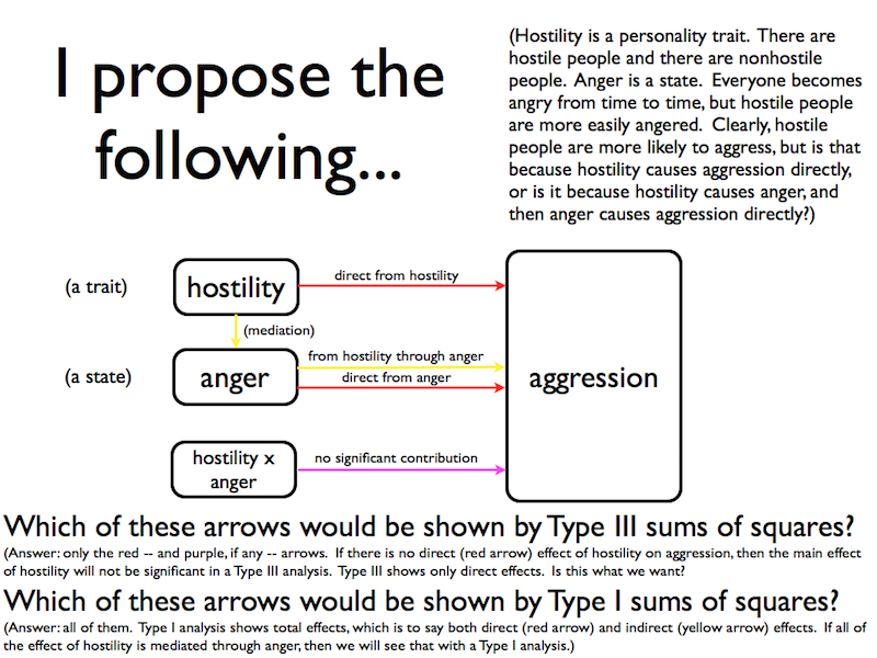
We suspect that there is a "flow of influence" (cause and effect) between hostility and anger. Hostile people are more easily angered. That's practically the very definition of hostility. In fact, we think it's possible that this might be the only way hostility can influence aggression.
We're going to use verbal aggression (verbag) as the DV. Let's begin with the Type III analysis. If you removed aovIII(), then you need to redo the source() command.
source("http://ww2.coastal.edu/kingw/psyc480/functions/aovIII.R") # only if you have to
And now...
aovIII(verbag ~ hostil * anger, data=X)
You should get the following output. (For those of you in the know, this is the same result you would get if you did this by standard multiple regression.)
Single term deletions

Model:
verbag ~ hostil * anger
             Df Sum of Sq    RSS    AIC F value Pr(>F)
-none-                    687.47 112.22
hostil        1    4.6724 692.14 110.45  0.2107 0.6494
anger         1   16.4610 703.93 111.05  0.7423 0.3955
hostil:anger  1    0.2482 687.72 110.23  0.0112 0.9164
Question 12. They're not called main effects anymore in regression, but I'm
going to call them that anyway because the idea is exactly the same. Is the main
effect of hostility on verbal aggression statistically significant? Summarize
the ANOVA. (Aha! Gotcha! There are no groups, so what is df.residuals? It is 31,
and you'll find out eventually why.)
Question 13. Is the main effect of anger on verbal aggression statistically
significant? Summarize the ANOVA.
Question 14. Is the interaction statistically significant? Summarize the
ANOVA.
Question 15. What did we find here?
Seriously? No effect of either hostility or anger on aggression? How is that even imaginable? (Refer to the above diagram again.) If hostility has only yellow arrows (indirect effects), then the Type III tests would have removed them. I'm a little surprised by anger. I would have expected a red arrow there (direct effect). But the bottom line is, we did the wrong test!
This is not a true experiment. Our IVs are quasi-experimental. The relationships between the IVs may not be "confounds," they may be legitimate effects. In fact, that's what we're proposing, so we don't want those effects stripped away by a Type III analysis. We want to see them, and that means Type I analysis. Provided we have our causal model correct, a Type I analysis will show total effects. (For regression-knowledgeable people, sequential regression shows total effects.) This is the causal model we are proposing.
hostility -> anger -> aggression
In this chain, hostility is the primary cause, i.e., it comes first in the chain. Therefore, it should be entered first into a Type I analysis.
aov.out = aov(verbag ~ hostil * anger, data=X)
summary(aov.out)
You should see this output.
             Df Sum Sq Mean Sq F value Pr(>F)
hostil        1  146.2  146.18   6.592 0.0153 *
anger         1  126.4  126.39   5.699 0.0233 *
hostil:anger  1    0.2    0.25   0.011 0.9164
Residuals    31  687.5   22.18
---
Signif. codes:  0 '***' 0.001 '**' 0.01 '*' 0.05 '.' 0.1 ' ' 1
The effect of hostility is now significant. Whether that is due to a red arrow (direct effect) or a yellow arrow (indirect effect) or possibly a combination of both, this analysis does not tell us (yet). The effect of anger is also significant. Because anger is entered last (2nd in this case) into the analysis, that must be due to arrows (red and yellow) going directly from anger to aggression. There are no more possible mediators in the model. (That is NOT to say that other mediators don't exist, but only that we haven't thought of them soon enough to include them in our little three-variable universe. And there is also that interaction term, but the interaction effect is so pathetically small that we can safely ignore it.)
Okay, now here is the really hard part of the logic, so read slowly and carefully. How might we try to show whether hostility has some direct effect on aggression or whether the entire effect of hostility is indirect (i.e., mediated through anger)? How about reversing the order in which the variables are entered into the Type I analysis? That would take the mediator of hostility away and show only direct effects of hostility, if any. If anger is entered first, it will gobble up any effect of hostility that is mediated through it and leave hostility with only its red arrow. (Read this paragraph over and over until you get it. This is important!)
aov.out2 = aov(verbag ~ anger * hostil, data=X)
summary(aov.out2)
             Df Sum Sq Mean Sq F value  Pr(>F)
anger         1  240.5  240.53  10.846 0.00248 **
hostil        1   32.0   32.04   1.445 0.23849
anger:hostil  1    0.2    0.25   0.011 0.91643
Residuals    31  687.5   22.18
---
Signif. codes:  0 '***' 0.001 '**' 0.01 '*' 0.05 '.' 0.1 ' ' 1
This suggests that there are no arrows, or at least no "significant arrows," going from hostility to aggression. To be honest, I'm not entirely convinced there is not a direct effect of hostility on aggression, but "we find no convincing evidence of such a direct effect in this analysis." Once the anger hog, feeding first, has eaten all of the total variability it can get, which would include anything coming through it from other variables (just because we got the model wrong doesn't mean the hog isn't going to feast on that variability anyway), there is very little if anything left over for hostility.
I'll cover how to do the Type II analysis in R in the practice problems and in the following video. Watch it carefully.