Today we review balanced factorial ANOVA from beginning to end. We'll enter the data at the command line, since there is not much of it. The source of the data is:
https://psych.unl.edu/psycrs/handcomp/hcbgfact.PDF
UNL is the University of Nebraska-Lincoln. The website describes the experiment but does not give a citation.
The data for this example are taken from a study that looked at the joint influence upon vocabulary test performance of the method used to study and the familiarity of the words. Five subjects were randomly assigned to each of four conditions of this factorial design (familiar words studied using definitions, familiar words studied using literature passages, unfamiliar words studied using definitions, and unfamiliar words studied using literature passages).
Here are the data in tabular form.
| study.type definition |
study.type literature |
|
| word.type familiar |
16, 16, 13, 12, 15 | 14, 14, 15, 12, 12 |
| word.type unfamiliar |
11, 10, 12, 11, 14 | 8, 6, 7, 9, 6 |
The DV was number of words recalled correctly on a 20-word vocabulary test (recall). Enter the following lines into R to get the data into a data frame in your workspace. I've left off the command prompts to make it easier to copy and paste these lines into R. (The dataset is also simple enoungh that you could do a lot of this by hand, if you're that masochistic.)
recall = c(16, 16, 13, 12, 15, 14, 14, 15, 12, 12, 11, 10, 12, 11, 14, 8, 6, 7, 9, 6)
You could also use scan() to enter these data, but you couldn't copy and paste them because scan() doesn't like commas.
Either way, I hope you remember what order those scores are in, i.e., which group each score is from, because you'll need that information to create the IVs. First, there are 10 scores from the familiar word.type, and then 10 scores from the unfamiliar word.type. So...
word.type = rep(c("familiar","unfamiliar"), each=10)
word.type = factor(word.type)
The second IV is going to be a little harder, because in our DV, we have 5 scores from definition study.type, then 5 scores from literature study.type, then 5 more scores from study.type definition, and finally 5 more scores from study.type literature. There is a way to get fancy with that, but I'm going to do it in a more clumsy but straightforward way.
study.type = rep(c("definition","literature","definition","literature"), each=5)
study.type = factor(study.type)
Now I'm going to put those variables into a data frame. As you know, we don't have to do this. We can use the variables from right in the workspace, but I'm going to put them into a data frame and then, to avoid confusion, erase them from the workspace.
vocab = data.frame(recall, word.type, study.type)
rm(recall, word.type, study.type)
Finally, I'm going to write the data out to a CSV file, just in case I want to use it again sometime. This is an optional step. It's here for those of you who want to know how to archive data you've entered in R. R will write the file to your working directory. If you don't know what that is, find out as follows.
> getwd()
[1] "/Users/billking"
That is the folder (directory) in which I will find my file after I write it. I could change that to the Desktop if I wanted to, but what the heck, I'll leave it. Just remember, if you want to know where R expects to find things you try to read in, or where it will write things, getwd() will tell you. Now I'll write the data frame as a plain text CSV file.
> write.csv(vocab, file="vocab.csv", quote=F, row.names=F)
The options quote=F and row.names=F are unnecessary, but setting them both to FALSE will give you a little cleaner CSV file. CSV is a universal file format because it is plain text. You can now open this file in almost anything, a text editor, a spreadsheet, just about any stat software on the planet worthy of the name. There is no proprietary formating, as there would be in an SPSS .sav file. The price is, any special declarations about the data are now lost, but R is usually clever enough to know what kind of variables you have without being told, unlike other stat software packages I might mention. If you want to save the whole shebang, just do save.image("vocab.RData"). This file will not open in anything but R, but all you have to do is double click it to open it.
A couple common errors (one of which I just made): Do NOT quote the data frame name! I.e., don't do write.csv("vocab", etc. That will work, but it will not write what you want it to write. The data frame is an object in your workspace. The names of objects in your workspace are never quoted. File names and directory pathways, on the other hand, are ALWAYS quoted. If you don't, R will look for something in your workspace with that name, won't find it, and will give you an error message. Data objects never quoted. File names always quoted.
Okay, END OF THE OPTIONAL STUFF!
Now let's see what we've got.
> ls()
[1] "vocab"
"vocab" is the data frame. Let's just print the whole thing to the R Console, since it's fairly small.
> vocab
   recall  word.type study.type
1      16   familiar definition
2      16   familiar definition
3      13   familiar definition
4      12   familiar definition
5      15   familiar definition
6      14   familiar literature
7      14   familiar literature
8      15   familiar literature
9      12   familiar literature
10     12   familiar literature
11     11 unfamiliar definition
12     10 unfamiliar definition
13     12 unfamiliar definition
14     11 unfamiliar definition
15     14 unfamiliar definition
16      8 unfamiliar literature
17      6 unfamiliar literature
18      7 unfamiliar literature
19      9 unfamiliar literature
20      6 unfamiliar literature
Remember, the numbers in the far left column are not part of the data. Those are row names supplied by R. Those were not included in your CSV file, because you set row.names=F. A note: They look like numbers, don't they? They are NOT numbers. They are names. More about this when it becomes necessary.
> summary(vocab)
     recall           word.type       study.type
 Min.   : 6.00   familiar  :10   definition:10
 1st Qu.: 9.75   unfamiliar:10   literature:10
 Median :12.00
 Mean   :11.65
 3rd Qu.:14.00
 Max.   :16.00
Suppose we didn't know that "vocab" is a data frame, or weren't sure. How could we find out what kind of object it is? Using summary() is one way. If you get the above sort of summary, you've got a data frame. Another way is this.
> class(vocab)
[1] "data.frame"
Question 1) What do we do first?
> with(vocab, table(word.type, study.type))
            study.type
word.type    definition literature
  familiar            5          5
  unfamiliar          5          5
What critical thing have we learned from this? How many subjects are in each of the groups?
Why do we need to use with()?
Question 2) How would you name this design?
> with(vocab, tapply(recall, list(word.type), mean))
  familiar unfamiliar
      13.9        9.4
> with(vocab, tapply(recall, list(study.type), mean))
definition literature
      13.0       10.3
Question 3) What means are these?
Question 4) Are these weighted or unweighted means?
Question 5) What effect is shown in the second pair of means?
> with(vocab, tapply(recall, list(word.type, study.type), mean))
           definition literature
familiar         14.4       13.4
unfamiliar       11.6        7.2
Question 6) What means are these?
Question 7) Are these means weighted or unweighted?
> with(vocab, tapply(recall, list(word.type, study.type), var))
           definition literature
familiar          3.3        1.8
unfamiliar        2.3        1.7
Question 8) The variances are not all the same. Does this mean that the
homogeneity of variance assumption has been violated?
> with(vocab, interaction.plot(word.type, study.type, recall, type="b", pch=c(2,16)))
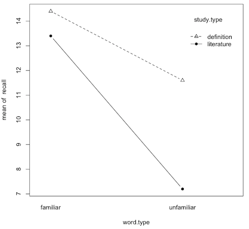
Question 9) What is this graph called (two names)?
Question 10) What effects are clearly shown on this graph? How?
10a) main effect of word.type (yes/no, explain):
10b) main effect of study.type (yes/no, explain):
10a) word.type-by-study.type interaction (yes/no, explain):
> aov.out = aov(recall ~ word.type * study.type, data=vocab)
> summary(aov.out)
                     Df Sum Sq Mean Sq F value   Pr(>F)
word.type             1 101.25  101.25  44.505 5.37e-06
study.type            1  36.45   36.45  16.022  0.00103
word.type:study.type  1  14.45   14.45   6.352  0.02273
Residuals            16  36.40    2.27
Question 11) Is the main effect of word.type statistically significant?
Summarize the results of the ANOVA? (Hint: Look at the p-values, because it's
possible some crafty professor erased the significance stars.)
Question 12) Is the main effect of study.type statistically significant?
Summarize the results of the ANOVA?
Question 14) Which of these effects is most interesting? Why?
> par(mfrow=c(2,2))  # sets the graphics window for four graphs
> plot(aov.out, 1:4)
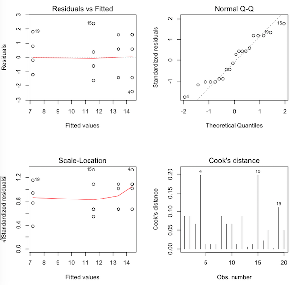
Question 15) What are these graphs called?
Question 16) Would you say the normal distribution assumption has been met
by these data? Why?
Question 17) Would you say the homogeneity of variance assumption has been met
by these data? Why?
Question 18) Would you say we have any problematic outliers in these data? Why?
Let's take a look at those three cases that have been flagged by R. To do this, we type the name of the data frame, and then inside square brackets, we indicate the rows and then the columns we want to see. We want to see rows 4, 15, and 19 (and here is where R really has the potential to confuse you, because those are row numbers, not row names, but okay, as long as row numbers and row names are the same, we won't have a problem). We put those row numbers inside of a vector (good rule of thumb to remember: in R, everything is a vector!), then type a comma, then indicate which columns we wish to see. We want to see all columns, so the shortcut method of telling R that is to leave that index blank.
> vocab[c(4,15,19), ]   # show rows 4, 15, and 19, and all columns (blank index)
   recall  word.type study.type
4      12   familiar definition
15     14 unfamiliar definition
19      9 unfamiliar literature
In each case, those are the values that are farthest from their group means, the most "extreme" values in the group. Nevertheless, they don't strike me as being extreme, so I'm happy with the "no problematic outliers" assumption.
A reminder:
> with(vocab, tapply(recall, list(word.type,study.type),mean))
           definition literature
familiar         14.4       13.4
unfamiliar       11.6        7.2
Question 19-22) What are the simple effects?Question 23) Because all the simple effects involve only two means, could we
use t-tests to test the simple effects? What would those t-tests be called?
Question 24) If there were simple effects with more than two means, what
test would we resort to?
Question 25) If we were going to do the Fisher LSD tests, what would be the
value of the pooled standard deviation? How do we get it?
What would be an even simpler way of getting the pooled standard deviation?
Okay, so how do we get se.meandiff for these tests?
Question 26) If we wanted a Bonferroni adjustment to the Fisher LSD p-values,
by what value would we multiple? Why?
Questions 27-38) Now complete the following table of tests. (Drop any irrelevant negative signs. Note: p values are from the Fisher LSD tests.)
| Tests of Simple Effects | |||||||
| Test | mean difference |
standard error |
t value | df | p value | significant by Fisher LSD test (yes/no) |
significant by Bonferroni test (yes/no) |
| study.type at familiar word.type | 27) | 0.954 | 1.05 | 16 | 0.309 | 28) | 29) |
| study.type at unfamiliar word.type | 30) | 0.954 | 4.61 | 16 | 0.000290 | 31) | 32) |
| word.type at definition study.type | 33) | 0.954 | 2.94 | 16 | 0.00961 | 34) | 35) |
| word.type at literature study.type | 36) | 0.954 | 6.50 | 16 | 0.00000732 | 37) | 38) |
Question 39) Why would it be pointless to do post hoc tests on the main
effects in a 2x2 ANOVA?
Question 40) Why is the standard error always the same in the
Fisher LSD/Bonferroni tests?
Question 41) Which of these tests is better in this case, Fisher LSD or
Bonferroni? Why?
We will use eta-squared as our effect size statistic. For that, we will need to get SS.total.
Question 42) What is SS.total? (Since there are only two decimal places
in the ANOVA summary table, two decimal places will do here.)
Questions 43-45) What are the following eta-squared values? (Three decimal places please.)
word.type: eta-sq =
study.type: eta-sq =
word.type-by-study.type: eta-sq =
Question 46) How would you evaluate the size of the interaction effect?
Subjects were given a 20-word list of vocabulary words to learn. Half of the subjects were given familiar words while the other half were given unfamiliar words. Half of each of those groups were given the definitions of the words while the other half were given a literature passage containing each word, thus creating a factorial design. After having time to study the words, the subjects were given a 20-word vocabulary test. Subjects learned significantly more of the familiar words than the unfamiliar words. They also learned significantly more words when given the definition as opposed to a literature passage. The negative effect of being given unfamiliar words was greater when subjects were given the words in a literature passage than when given definitions.
Question 47) Is this a reasonable conclusion describing the results of
this study (yes/no)?