Psyc 480 -- Dr. King
Mixed Factorial Designs
This will be our one foray into mixed factorial designs, because you should know something about them.
Clear your workspace, then get the following data set from the website.
file = "http://ww2.coastal.edu/kingw/psyc480/data/serotonin.txt"
Hill = read.table(file=file, header=T, stringsAsFactors=T)
summary(Hill)
You will also need the following function.
source("http://ww2.coastal.edu/kingw/psyc480/functions/mixaov.R")
When you examine your workspace, it should look like this.
> ls()
[1] "file"   "Hill"   "mixaov"
Here is a description of the data taken from the data set itself.
# serotonin.txt
# Data from Ben Hill's (now Dr. Hill, Ph.D.) Psyc 497 study (Fall 1999).
# Subjects came to the lab late in the afternoon, and were given the
# Sensation Seeking Survey, then ate a meal of either chicken or
# pasta, waited 1 hr., then took the Sensation Seeking Survey a
# second time. The variable "meal" is obvious. The variables "pretest"
# and "posttest" give the premeal SSS score and postmeal SSS score,
# respectively. This is a wide format data frame with one subject per
# row. The same data occur in serotonin.csv in long format. The point:
# meals high in carbohydrates, such as pasta, supposedly increase
# tryptophan uptake into the brain, increasing brain levels of serotonin.
# Did this have an effect on the sensation seeking scores?
In mixed factorial designs, some of the factors (IVs) are measured between groups and others are measured within subjects (or blocks). These designs can become very complex, but we will restrict ourselves to cases in which there are only two factors, one between and one within.
Question 1. In the Hill data frame, which variable is the one being measured
between groups?
Hint: Type Hill and press Enter at the command prompt. The data frame is small enough to print out in the Console window. (Ben had to cook dinner for these people after all, so there weren't going to be a whole lot of subjects!) If you look at the data frame, there is one variable where some subjects got one thing and other subjects got another thing (between groups factor), whereas in the other columns, every subject got this and that (within subjects factor).
We are still in the realm of simple experimental designs, in which it is easy to put every subject on a line (wide or short format) in the data frame. This is the way I, personally, would prepare the data. Unfortunately, the aov() function in the R base packages cannot handle the data in this format.
If you've become enamored of R, there are optional packages you can download that will handle wide format data frames. In fact, there are thousands of optional packages you can download and add to your R installation, which will do just about any statistical procedure you can imagine (and many you can't), as well as a lot of things that aren't statistical, but we cannot download those packages onto computers in the lab or library, so I prefer to stick with the base packages for teaching purposes.
However, as you already know, there are a few things that are conspicuously absent from the base packages, such as an easy way to do Type III sums of squares in an unbalanced factorial design, so I've written my own functions for those. (The first one was sum of squares! It still irks me that there is no SS() function in the R base packages, but the function is so easy to create at the command line that the R people can be excused for that one.) I also wrote the rmsaov.test() function to handled single-factor repeated measures designs when the data are in a wide (short) format data frame.
This data frame would be a single-factor data frame if it weren't for that first column. In fact, we can test columns 2 and 3 against each other with a related measures t-test.
t.test(Hill$pretest, Hill$posttest, paired=T)
Question 2. By t-test, was there a significant difference between pretest and
posttest scores on the SSS (yes/no)?
Question 3. What was the p-value?
Question 4. Did SSS scores increase or decrease from pretest to posttest, on
the average?
Optional part. If you want to learn something about the relationship between the related measures t-test and repeated measures ANOVA, fetch the rmsaov.test() function, and try this.
> rmsaov.test(as.matrix(Hill[,2:3])) # just columns 2 and 3 of Hill
End of optional part.
This is the simplest possible case because there are only two levels of each of the factors. This would be called a 2x2 mixed factorial design. So here's a question for you. Since there are only two levels of the repeated measures factor, why can't we just calculate a change score (as we would in the related measures t-test), and then test the between groups factor by doing an independent groups t-test against the change scores? Answer: We can do exactly that!
Hill$change = Hill$posttest - Hill$pretest
t.test(change ~ meal, data=Hill, var.eq=T)
Question 5. What was the average change in SSS scores in the chicken group?
Question 6. What was the average change in SSS scores in the pasta group?
Question 7. By t-test, was there a significant difference in mean change scores
between the chicken and pasta groups (yes/no)?
Question 8. What was the p-value?
Question 8a. Are you surprised by the direction this effect went in, i.e.,
that an increase in brain serotonin increased sensation seeking scores? If
you are, then settle down, because we have no reason to believe that this is
anything other than random noise. However, suppose that we had predicted
that the effect would go in this direction, and had stated the alternative
hypothesis appropriately as a directional hypothesis, and tested it as such.
What would have been the p-value from the t-test?
So why aren't we done? There appears to be no significant effect of the repeated measures factor, and there appears to be no significant effect of the between groups factor. Why aren't we done?
Question 9. It's a factorial design. What effect have we NOT tested for?
If you look at the Hill data frame, you'll notice a column has been added to it called "change". We can live with that, so we're going to leave it. Unlike the rmsaov.test() function, for the mixaov() function, the data frame will not be converted to a matrix, and the function will just ignore extraneous columns. So let's run it.
You need to tell the mixaov() function what the name of the data frame is, you need to tell it what column of the data frame contains the between groups factor, and you need to tell it what columns of the data frame contain the within subjects factor. Since there are more than one column that contain the within subjects factor, those column numbers have to be entered as a vector using c(). It looks like this. I'll also show the output, because I want to discuss it in some detail.
> mixaov(Hill, betw.IV.col=1, within.IV.col=c(2,3))

Error: subjects
          Df Sum Sq Mean Sq F value Pr(>F)
betw.IV    1   40.1   40.11   0.509  0.486
Residuals 16 1259.8   78.74

Error: subjects:within.IV
                  Df Sum Sq Mean Sq F value Pr(>F)
within.IV          1  2.778   2.778   2.174   0.16
betw.IV:within.IV  1  2.778   2.778   2.174   0.16
Residuals         16 20.444   1.278
Here's what happens. In a mixed factorial design, the ANOVA not only has to partition the explained variability into its various effects (the usual three of them in the case of a two-factor design), but it also has to partition the unexplained variability into separate error terms for the between groups IV and the within subjects IV (and any effect containing the within subjects IV). So the first table shows the test on the between groups IV (and it's up to you to remember which one that is), with its own error (Residuals) term, which is variability due to subjects. The second table shows the tests on the within subjects IV and any effect containing that IV, with its own error term, which is variability due to a subjects-by-within.IV interaction. This is very similar to what happens in a single-factor repeated measures design, EXCEPT an additional factor is pulled out of the error term (the between groups factor). Because of that, these tests are also exquisitely sensitive to violations of homogeneity of variance and sphericity, but no tests for that appear in this output. You get the ANOVA summary table, period.
Well, not quite "period". The mixaov() function has added two things to your workspace. Let's look.
> ls()
[1] "aov.mix"        "dataframe.long" "file"           "Hill"           "mixaov"
There is an aov() output object called aov.mix (similar to what we've been calling aov.out in the past). You can recall the above summary table at any time by typing summary(aov.mix) at the command prompt.
There is also something called dataframe.long. The mixaov() function has converted the wide (short) format data frame into a "proper" long format data frame. (The wide format data frame is also still there, unaltered.) The reason for this is that there are a number of important R functions, such as tapply() and interaction.plot(), that won't work properly with a wide format data frame. Well, now you can use them. But let's not get ahead of ourselves.
Question 10. As you would expect for a two-factor design, three effects have
been tested, the effect of the between groups factor, the effect of the within subjects
factor (both still called main effects), and the interaction between them. Were
any of those effects statistically significant?
Let's look at the long format data frame.
> head(dataframe.long)   # first six rows
  DV within.IV betw.IV subjects
1 18   pretest chicken       S1
2 13   pretest chicken       S2
3 18   pretest chicken       S3
4 15   pretest chicken       S4
5 22   pretest chicken       S5
6 32   pretest chicken       S6
In a long format data frame, there must be a subjects identifier, and that is in the last column. Now also, each of the variables has its own column: DV, within.IV, and between.IV. You might expect this in a "proper" data frame. What this means, however, is that rows in the data frame are no longer defined by subjects but by values of the DV, and since each subject has more than one of those, each subject will have multiple rows in the data frame. The first row is subject S1, a chicken subject, but only his (or her) pretest score appears. S1's posttest score will be in another row. In fact, it's in row 19. (How did I know that? I looked!)
> dataframe.long[c(1,19),]   # rows 1 and 19, all columns
   DV within.IV betw.IV subjects
1  18   pretest chicken       S1
19 15  posttest chicken       S1
If I intended to so something with this data frame, the first thing I would want to do is change those column names.
colnames(dataframe.long) = c("SSS.score","time","meal","subjects")
head(dataframe.long)
Ahhh! I feel so much better. I also want to change the name of the data frame so when I look at my workspace, I recognize what it is a week from now (or five minutes from now for that matter). That involves copying the data frame to a new name and then removing the old one.
Hill.long = dataframe.long
rm(dataframe.long)
ls()
Now, using tapply(), you can fill in the following table of cell means. Two decimal places will be sufficient. (Some of you had to ask me how to do this on the last graded exercise. I was not pleased! Where have you been?) Okay, how? (I'm rolling my eyes bigtime here! Remember this! I'm not answering this question again!)
| pretest | posttest | |
| chicken | 11) | 12) |
| pasta | 13) | 14) |
We can also get an interaction (or profile) plot. I'll give you this one.
with(Hill.long, interaction.plot(time, meal, SSS.score, type="b", pch=1:2))
Gee! It looks like there are effects there. What happened to them? (Hint: Look at the scale on the vertical axis. All the means are very similar.)
Problem Two.
Let's look at another very similar data set. First, we'll clean up the workspace. BUT don't delete the mixaov() function. Or if you have already, source it in again.
> ls()
[1] "aov.mix"   "file"      "Hill"      "Hill.long" "mixaov"
> rm(aov.mix,file,Hill,Hill.long)
> data(anorexia, package="MASS")   # a built-in dataset (comes with the download)
> ls()
[1] "anorexia" "mixaov"
> summary(anorexia)
  Treat        Prewt           Postwt
 CBT :29   Min.   :70.00   Min.   : 71.30
 Cont:26   1st Qu.:79.60   1st Qu.: 79.33
 FT  :17   Median :82.30   Median : 84.05
           Mean   :82.41   Mean   : 85.17
           3rd Qu.:86.00   3rd Qu.: 91.55
           Max.   :94.90   Max.   :103.60
These data are from the "anorexia" built-in data set in R's MASS library. They can also be found in Hand et al. (1993), A Handbook of Small Datasets. (You can pick up a copy at amazon for a mere $220 if you're interested. Even I'm not that interested!) The data are from a study on the treatment of anorexia in young women. Three different treatment methods were used, CBT (cognitive behavioral therapy), Cont (no treatment control), and FT (family therapy). That's clearly the between groups factor, and it's in the first column of the data frame. Then we have weight in pounds before treatment (Prewt) and weight in pounds after treatment (Postwt). This is the within subjects factor, as each woman was measured twice. Those measurements are in columns 2 and 3. (Each row of the data frame is one subject, so this is a wide format data frame.) I have no more details than that. I have never seen this study published.
If I calculate means, I'd like to see the control mean first, so I'm going to relevel that variable.
> anorexia$Treat = relevel(anorexia$Treat, ref="Cont")
Now these will give a somewhat tidier result. It won't change the means at all, but the output will look at little prettier.
> with(anorexia, tapply(Prewt, Treat, mean))
    Cont      CBT       FT
81.55769 82.68966 83.22941
> with(anorexia, tapply(Postwt, Treat, mean))
    Cont      CBT       FT
81.10769 85.69655 90.49412
This is a 3x2 mixed factorial design with repeated measures on the second factor. So in the factorial structure of this design, those are cell means. Looking at those cell means and imagining them plotted in an interaction plot (or sketched out on a piece of scrap paper), which of the following effects would you say exist?
| main effect of treatment type | 15) |
| main effect to time (pre vs. post) | 16) |
| treatment type by time interaction | 17) |
Now we'll do the ANOVA and see.
> mixaov(anorexia, betw.IV.col=1, within.IV.col=c(2,3))

Error: subjects
          Df Sum Sq Mean Sq F value  Pr(>F)
betw.IV    2    644   322.1   6.201 0.00334 **
Residuals 69   3584    51.9
---
Signif. codes:  0 '***' 0.001 '**' 0.01 '*' 0.05 '.' 0.1 ' ' 1

Error: subjects:within.IV
                  Df Sum Sq Mean Sq F value  Pr(>F)
within.IV          1  275.0  275.01   9.704 0.00268 **
betw.IV:within.IV  2  307.3  153.66   5.422 0.00650 **
Residuals         69 1955.4   28.34
---
Signif. codes:  0 '***' 0.001 '**' 0.01 '*' 0.05 '.' 0.1 ' ' 1
Were you right? Let's clean up the long format data frame and draw an interaction plot.
> ls()
[1] "anorexia" "aov.mix" "dataframe.long" "mixaov"
> head(dataframe.long)
DV within.IV betw.IV subjects
1 80.7 Prewt Cont S1
2 89.4 Prewt Cont S2
3 91.8 Prewt Cont S3
4 74.0 Prewt Cont S4
5 78.1 Prewt Cont S5
6 88.3 Prewt Cont S6
> colnames(dataframe.long) = c("weight","time","treatment","subjects")
> anorexia.long = dataframe.long
> rm(dataframe.long)
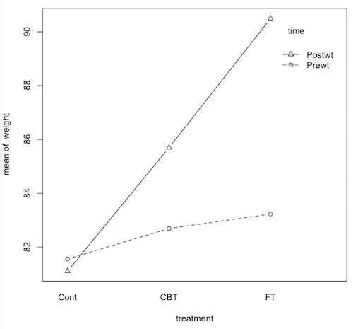
> with(anorexia.long, interaction.plot(treatment,time,weight,type="b",pch=1:2))
Finally, we'll do the ANOVA in two different ways. First, from the wide format data frame...
(See above. We've already done this!)
And now I'll show you how to do it from the long format data frame, in case you ever need to know that, which you will not in this class. The ANOVA is specified in the usual fashion for a two-factor ANOVA inside the aov() function, but there is one added element. You have to tell R which is the repeated measures factor. That is done by adding +Error(name.of.subjects.identifier/name.of.within.IV) to the aov formula. In this case, it looks like this.
> aov.out = aov(weight ~ treatment * time + Error(subjects/time), data=anorexia.long)
> summary(aov.out)

Error: subjects
          Df Sum Sq Mean Sq F value  Pr(>F)
treatment  2    644   322.1   6.201 0.00334 **
Residuals 69   3584    51.9
---
Signif. codes:  0 '***' 0.001 '**' 0.01 '*' 0.05 '.' 0.1 ' ' 1

Error: subjects:time
               Df Sum Sq Mean Sq F value  Pr(>F)
time            1  275.0  275.01   9.704 0.00268 **
treatment:time  2  307.3  153.66   5.422 0.00650 **
Residuals      69 1955.4   28.34
---
Signif. codes:  0 '***' 0.001 '**' 0.01 '*' 0.05 '.' 0.1 ' ' 1
Here's a sad fact. In the base packages, the Tukey HSD test has not been implemented for designs with a +Error term. There are various ways we could do post hoc tests here, but let's not get caught up in it. The interaction is significant, so that's the interesting effect.
Which of the following statements are correct?
Question 18. The fact that the dashed line on the interaction plot is not
flat means that the groups did not start out equal before treatment (correct/incorrect/can't say)?
Question 19. Both the FT group and the CBT group had significant weight gain,
on the average, due to these treatments? (correct/incorrect/can't say)
Question 20. In general, the posttreatment body weights where higher than
the pretreatment weights, but the difference was largest in the FT group, less
than half as large in the CBT group, and didn't occur at all in the control
group. Is this a correct description of the interaction (correct/incorrect/can't say)?
You will not have to do one of these on the next graded exercise, but you may need to understand what it is and how to interpret it, so make sure you ask questions if there's something you don't understand about it.