In this exercise, we are going to discuss blocking variables in experimental designs. If that sounds like something new, it is new in name only. Sometimes instead of having measures repeated within subjects, we have a single, unique subject in every condition of our experiment, but similar subjects are grouped together by some similarity that they have to each other. That similarity factor is called a blocking variable. I should probably hurry up and give an example!
Suppose we want to measure the effect of teaching method on student learning. First, of course, we need a measure of student learning to serve as our DV. We will do that by giving the students a comprehensive final exam at the end of the course. Exam score will be the DV.
The treatment will be teaching method, and I have three in mind: lecture, discussion, and virtual. That's our IV.
There is another variable, however, that influences student performance, and that is intelligence. Intelligence probably (certainly!) will have a greater impact on our DV than teaching method will, so we want to make sure we have some control over that. We don't want a lot of uncontrolled noise in out dependent variable. Our control will be to make intelligence a blocking variable.
We have 18 students who are going to participate as subjects in our study. We give them some sort of intelligence test and then we group them together according to the IQ measure. Students with similar IQs are put in the same group, or block. Our design table ends up looking like this.
| virtual | discussion | lecture | |
| IQ.91-95 | n = 1 | n = 1 | n = 1 |
| IQ.96-100 | n = 1 | n = 1 | n = 1 |
| IQ.101-105 | n = 1 | n = 1 | n = 1 |
| IQ.106-110 | n = 1 | n = 1 | n = 1 |
| IQ.111-115 | n = 1 | n = 1 | n = 1 |
| IQ.116-120 | n = 1 | n = 1 | n = 1 |
Our blocks are the IQ ranges, and in each of those blocks we have three subjects. Within a block, it is important that the three subjects are randomly assigned to a teaching method. Because of this random assignment within blocks, this design is sometimes called a randomized blocks design. (I personally find that name a little confusing, but it's probably the more common name for this kind of design, so you should remember it.)
What's the difference between this and a factorial design? Not a lot! There is no replication within the cells. That is, in every cell, n = 1. If we had multiple subjects (n > 1) in every cell, this would be a factorial design.
In this case, however, the blocks are like subjects in a repeated measures design, and that's how the data will be analyzed. Obviously, we couldn't use the same subjects over again in the three different teaching methods, so we did the next best thing, we matched up subjects within blocks of similar IQ. We usually wouldn't do a significance test on the blocking variable, because it's just there as a control, but we can if we want to.
Question: What other experimental design do you know of that is similar to this?
Question: What other data have we seen previously that is very similar to this?
So our planned analysis is repeated measures ANOVA in which blocks are like "subjects," and let's also do TukeyHSD tests post hoc if the main effect of teaching method turns out to be significant. Ready to go? Let's get some data!
| virtual | discussion | lecture | |
| IQ.91-95 | 84 | 85 | 85 |
| IQ.96-100 | 86 | 86 | 88 |
| IQ.101-105 | 86 | 87 | 88 |
| IQ.106-110 | 89 | 88 | 89 |
| IQ.111-115 | 88 | 89 | 89 |
| IQ.116-120 | 91 | 90 | 91 |
Aside: I have to warn you, I got these data online. If you're ever tempted to fake some data, DON'T! But if you can't help yourself, do a better job of it than this! It's fairly easy to detect fake data, and if you're found out, your career is over. In science and academia, that is a mortal sin. You'd be better of punching your boss. (Just joking! Don't punch your boss!) Enough said.
This is a small dataset, so we are going to enter it by hand.
Strictly speaking, you do not need R to complete this exercise, but I would use it if I were you. It will make future exercises much easier and much less prone to error. (Hint!) I'm going to show you a way to get the data in that will work well for smaller datasets. Personally, I would do this in a script window, but whatever floats your boat. But doing it in a script window (File > New Script or New Document) will allow you to edit it if you make a mistake. If you make a mistake typing it into the Console window, you start over again. I showed you how to use a script window in a previous video.
If you want to get these data into R, here's how you can do it quickly. You'll have to watch your typing because everything is crucial here, but if you're careful enough, this will work. I'm going to enter the data directly into a matrix in short format. Then I'm going to convert the matrix to a data frame. (Remember, all that spacing is optional, but it helps keep things straight. Also, there is a minor and fairly unimportant error in data entry shown in the image. Can you spot it?)
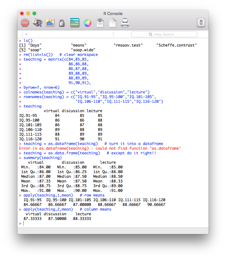
Here is a copy-and-pasteable version of the data entry for those without the nerve to try to get the typing correct (but seriously, I would practice this if I were you because you never know when you might have to do it). First, clear your workspace using either a menu or a command line function.
# ---------begin copying here---------
teaching = matrix(c(84,85,85,
                    86,86,88,
                    86,87,88,
                    89,88,89,
                    88,89,89,
                    91,90,91),
    byrow=T, nrow=6)
colnames(teaching) = c("virtual","discussion","lecture")
rownames(teaching) = c("IQ.91-95","IQ.96-100","IQ.101-105",
                       "IQ.106-110","IQ.111-115","IQ.116-120")
teaching = as.data.frame(teaching)
# ---------end copying here-----------
Looking at the row means, would you say there is going to be a significant main effect of the blocking variable (IQ)? (Hint: a matrix must always be all numeric, but a data frame doesn't have to be. This one is, so the apply() function will still work: apply(teaching,1,mean).)
Is this an effect that we're interested in?
Looking at the column means, would you say there is going to be a significant main effect of teaching method?
Would an IQ-by-teaching method interaction be interesting?
Now I'm going to get the rmsaov.test() function from the website.
source("http://ww2.coastal.edu/kingw/psyc480/functions/rmsaov.R")
And now we might as well run it.
rmsaov.test(as.matrix(teaching))

	Oneway ANOVA with repeated measures

data:  as.matrix(teaching)
F = 4.4286, df treat = 2, df error = 10, p-value = 0.04194

  MS.error   MS.treat   MS.subjs
 0.3888889  1.7222222 12.8555556

Treatment Means
   virtual discussion    lecture
  87.33333   87.50000   88.33333

HSD.Tukey.95
   0.9869791

Compound Symmetry Check (Variance-Covariance Matrix)
            virtual discussion  lecture
virtual    6.266667        4.4 4.666667
discussion 4.400000        3.5 3.400000
lecture    4.666667        3.4 3.866667

Estimated Greenhouse-Geisser Epsilon and Adjusted p-value
   epsilon   p-adjust
0.91829085 0.04734859
Here are some questions for you to answer from the output.
Everything you need to fill in a conventional ANOVA table is in the output above, so do it! Use the ✓ buttons to check your work.
| Source | df | SS | MS | F | p.value |
| IQ blocks | |||||
| teaching method | |||||
| error | |||||
| total |
HSD.Tukey.95 is the Tukey honestly significant difference for alpha=0.05. Any difference between two means that is this large or larger is signficant at the 0.05 level. Using this number and the treatment means, we can reconstruct the same table that we would normally get from TukeyHSD(aov.out) after an ANOVA on a long format data frame (except for the p-values). Below is the skeleton of such a table. As you enter values into this table, you can check them by clicking the ✓ button.
As you are entering values into this table, rounding them accurately to four decimal places should be sufficient to avoid any untoward rounding error. The first column, diff, is just the difference between the two means of the conditions involved in the comparison. Calculate those and put them into the first column of the table.
The next two columns are the lower and upper limits of a 95% confidence interval around the mean difference in column one. They are calculated as follows:
To do these calculations, use diff from column one and HSD.Tukey.95 from the ANOVA output above.
In the last column, R would write p-values. We can't get those (without a lot of pain). So if the mean difference in column one is not signicantly different from 0, write "ns" in the last column. If the mean difference in column one is significantly different from 0, write "p < 0.05" in the last column. Why 0.05? Because that's the alpha level that HSD.Tukey.95 was calculated for. Now I know someone is going to ask, "How do we tell if it's significant or not?" Don't! You should know the answer to that. If the CI95% does not include 0, then we are 95% confident that the true mean difference in the population is not 0. You take it from there.
| diff | lwr | upr | p adj | |
| discussion-virtual | ||||
| lecture-virtual | ||||
| lecture-discussion |
What is the value of eta-squared for teaching method?
Evaluate.
You had to be able to get SS.treat and SS.total to solve that one, but you should be able to do that by now. You had to do it to get the conventional ANOVA table.
From the information you already have, is it possible to get a test on the blocking variable? Get an F-statistic for this test.
Is one teaching method better than the others (according to these results)?
We could also have used the "treatment-by-subjects" method of doing the ANOVA in R if we'd had a long format data frame. There is a way to get there from here, but it requires a little work.
> ls()
[1] "rmsaov.test" "teaching"
> teaching
           virtual discussion lecture
IQ.91-95        84         85      85
IQ.96-100       86         86      88
IQ.101-105      86         87      88
IQ.106-110      89         88      89
IQ.111-115      88         89      89
IQ.116-120      91         90      91
>
> scores = c(teaching$virtual, teaching$discussion, teaching$lecture)
> method = rep(c("virtual", "discussion", "lecture"), each=6)
> method = factor(method)
> ### Nothing new there. You've seen it before.
> ### Here's the tricky bit!
> blocks = rownames(teaching)     # get the rownames as block names
> blocks = rep(blocks, times=3)   # repeat 3 times, once for each condition
> blocks = factor(blocks)         # make it a factor
> ls()
[1] "blocks"      "method"      "rmsaov.test" "scores"      "teaching"
> ### The long variables are all in your workspace,
> ### not in a data frame, so...
> aov.out = aov(scores ~ blocks + method)   # remember, + not *
> summary(aov.out)
            Df Sum Sq Mean Sq F value   Pr(>F)
blocks       5  64.28  12.856  33.057 6.59e-06 ***
method       2   3.44   1.722   4.429   0.0419 *
Residuals   10   3.89   0.389
---
Signif. codes:  0 '***' 0.001 '**' 0.01 '*' 0.05 '.' 0.1 ' ' 1
>
> ### And finally...
> Tukey.HSD(aov.out, which="method")
Error in Tukey.HSD(aov.out, which = "method") :
  could not find function "Tukey.HSD"
> ### And finally (this time we'll do it right)...
> TukeyHSD(aov.out, which="method")
  Tukey multiple comparisons of means
    95% family-wise confidence level

Fit: aov(formula = scores ~ blocks + method)

$method
                         diff        lwr         upr     p adj
lecture-discussion  0.8333333 -0.1536457  1.82031238 0.0996681
virtual-discussion -0.1666667 -1.1536457  0.82031238 0.8898461
virtual-lecture    -1.0000000 -1.9869791 -0.01302095 0.0471259
Compare this to the result you calculated above.
What other post hoc test might have been done here?
Here's how you would do that test in R, given that you have the long variables in your workspace. (The tabled values are p-values in case you need a reminder of that.) You can see that we are now finding significant differences between lecture and both discussion and virtual.
pairwise.t.test(scores, method, p.adjust.method="none", paired=T)

	Pairwise comparisons using paired t tests

data:  scores and method

        discussion lecture
lecture 0.042      -
virtual 0.695      0.041

P value adjustment method: none
Would it be fair now to say, "Well, that's what I should have done in the first place, so I'm going to report those results"?
Fishing for statistics is when you do a whole bunch of statistical tests and then cherry-pick the ones you like. That invalidates the p-values in all the tests. That's not to say that people don't do it, but it is a very bad practice. Why bother doing statistical tests if you're not going to use them properly? Frankly, I would have used these tests myself, but I would have to have decided that in advance and then stuck with my decision. They don't tell you to make these decisions in advance for nothing. Your p-values depend on it!
By the way, these are just paired t-tests. They are not Fisher-LSD-like tests. They do not use a pooled standard deviation or degrees of freedom from the ANOVA. From the short (wide) format data frame, you could also have done these tests as follows.
t.test(teaching$lecture, teaching$discussion, paired=T)
t.test(teaching$lecture, teaching$virtual, paired=T)
t.test(teaching$discussion, teaching$virtual, paired=T)
If we had done a Bonferroni adjustment to the p-values from the t-tests, how many of the differences would still have been significant?
Hint!
pairwise.t.test(scores, method, p.adjust.method="bonferroni", paired=T)
Any questions?