I would be remiss if I didn't tell you that not everyone does hierarchical regression for the reason I (and Keith) have outlined. Sometimes hierarchical regression is done to see how much adding a certain variable or block of variables adds to R-squared without any implication of a flow of cause and effect. This could also be done with a standard multiple regression, but since it does involve comparing two or more sequential models, I suppose it is hierarchical regression in that sense. I found an example of that here, which I am going to borrow. The R command given on that page to download the data didn't work for me, so I downloaded the dataset in my browser and put it on my Desktop. If you want to follow along in R, I'll show you how you can do it using the R script window to enter the data.
To get the data:
If that worked, you should be able to do this. If it did not work, try copying
and pasting these two commands:
file="https://ww2.coastal.edu/kingw/psyc480/text/pets_and_happiness.txt"
PETS=read.csv(file=file,stringsAsFactors=T)
> ls()
[1] "PETS"
> summary(PETS)
   happiness         age           gender      friends           pets
 Min.   :1.00   Min.   :20.00   Female:39   Min.   : 1.00   Min.   :0.0
 1st Qu.:3.75   1st Qu.:24.00   Male  :61   1st Qu.: 5.00   1st Qu.:0.0
 Median :4.00   Median :25.00               Median : 7.00   Median :1.0
 Mean   :4.46   Mean   :25.37               Mean   : 6.94   Mean   :1.1
 3rd Qu.:5.00   3rd Qu.:27.00               3rd Qu.: 8.25   3rd Qu.:2.0
 Max.   :9.00   Max.   :30.00               Max.   :14.00   Max.   :5.0
Happiness is measured on some sort of psychological scale. Age and gender are obvious, although notice the restricted range of age. Friends and pets are counts of "how many" for each subject. I don't like the way "gender" is coded, so we're going to change it to a dummy coding. (I was tempted to say we're going to dummify it, but I didn't want anyone to be confused.)
> PETS$gender = as.numeric(PETS$gender) - 1
> summary(PETS)
   happiness         age            gender        friends           pets
 Min.   :1.00   Min.   :20.00   Min.   :0.00   Min.   : 1.00   Min.   :0.0
 1st Qu.:3.75   1st Qu.:24.00   1st Qu.:0.00   1st Qu.: 5.00   1st Qu.:0.0
 Median :4.00   Median :25.00   Median :1.00   Median : 7.00   Median :1.0
 Mean   :4.46   Mean   :25.37   Mean   :0.61   Mean   : 6.94   Mean   :1.1
 3rd Qu.:5.00   3rd Qu.:27.00   3rd Qu.:1.00   3rd Qu.: 8.25   3rd Qu.:2.0
 Max.   :9.00   Max.   :30.00   Max.   :1.00   Max.   :14.00   Max.   :5.0
The coding for "gender" is now 0=Female and 1=Male. I've already looked at scatterplots. They are kind of goofy looking (take a look) because all of these variables are integers (whole numbers). I didn't see any reason to be concerned, so let's move along.
> cor(PETS)
            happiness         age     gender     friends        pets
happiness  1.00000000 -0.16091772 0.03884059  0.32424344  0.29948447
age       -0.16091772  1.00000000 0.07760442 -0.02097324 -0.03786638
gender     0.03884059  0.07760442 1.00000000  0.01299759  0.33105816
friends    0.32424344 -0.02097324 0.01299759  1.00000000  0.11941881
pets       0.29948447 -0.03786638 0.33105816  0.11941881  1.00000000
What two things must be true to get this last command to work? The critical value of r (from the table at the webpage) is about 0.2, so which correlations are significantly different from zero? What does it mean that the happiness-pets correlation is positive? What does it mean that the gender-pets correlation is positive?
The problem is one of finding the determinants of happiness. We have four possible predictors: age, gender, friends, and pets. Previous research has shown that number of friends is an important determinant of happiness. We now want to find out what the effect of pets is. Adding pets to a regression model will increase R-squared, of course, but by how much? Will it alter the effect of friends? And will the increase in R-squared be statistically significant?
We're going to run three sequential models:
The first two models will replicate a previous finding, that after age and gender is accounted for, friends is a significant predictor of happiness. The third model will add pets to see if it improves the model after accounting for age, gender, and friends. No flow of influence, or cause and effect, is implied between the predictors. Of course, we're also going to want to report some descriptive statistics.
> apply(PETS, 2, mean)
happiness       age    gender   friends      pets
     4.46     25.37      0.61      6.94      1.10
> apply(PETS, 2, sd)
happiness       age    gender   friends      pets
1.5597203 1.9728204 0.4902071 2.6316642 1.1763666
> lm.0 = lm(happiness ~ 1, data=PETS)
> lm.1 = lm(happiness ~ age + gender, data=PETS)
> lm.2 = lm(happiness ~ age + gender + friends, data=PETS)
> lm.3 = lm(happiness ~ age + gender + friends + pets, data=PETS)
Done! And let's see those SPSS people do it that fast! They're still clicking their way through menus! Okay, so what the heck is lm.0, you may be wondering (hopefully, are wondering). The formula happiness~1 regresses happiness on the intercept only. We'll see the point of this shortly.
If we wanted to see if pets adds significantly to the model, isn't that last regression the only one we really need?
If we wanted to see if pets alters the effect of friends in the model, isn't that last regression the only one we really need?
Now I'm going to display the results in a way that is frequently (but not universally) done in journal articles, after which, we'll look at a real example from the literature.
| TABLE 1. HIERARCHICAL REGRESSION OF PREDICTORS OF HAPPINESS |
|||
| Predictor variables | Regression 1 | Regression 2 | Regression 3 |
| Age | -0.13 | -0.12 | -0.11 |
| Gender (0=Female, 1=Male) | 0.16 | 0.15 | -0.14 |
| Number of Friends | 0.19** | 0.17** | |
| Number of Pets | 0.36** | ||
| R2 | 0.03 | 0.13 | 0.20 |
| R2 change | 0.03 | 0.10** | 0.07** |
| *p < .05; **p < .01; ***p < .001 | |||
Okay, calm down! It's not that hard. The numbers in the columns labeled Regression are regression coefficients, which, of course, I got from:
> summary(lm.1)
> summary(lm.2)
> summary(lm.3)
I did not show the output of those commands here. Look at it on your own screen and compare to the table. Each coefficient is marked with significance stars (if p<.05), and the key to what those stars mean is at the bottom of table. The R-squared values also come from the output of those commands. The change values were obtained by subtraction, but not of these severely rounded values. I used the values in the outputs of the above commands. Journal editors are not happy when you don't round things fairly severely. Here, we are rounding to two decimal places, which ought to keep our editor happy, but we have to be careful about using rounded values for further calculations. See Table 3 in the Park, et al, article for an example.
The significance of the change values I got as follows. But notice, since lm.2 and lm.3 consisted of the addition of a single variable, I could also have gotten that from the summary() outputs. The following method should be used when blocks of variables are being added.
> anova(lm.0, lm.1)
Analysis of Variance Table

Model 1: happiness ~ 1
Model 2: happiness ~ age + gender
  Res.Df    RSS Df Sum of Sq      F Pr(>F)
1     99 240.84
2     97 233.97  2    6.8748 1.4251 0.2455

> anova(lm.1, lm.2)
Analysis of Variance Table

Model 1: happiness ~ age + gender
Model 2: happiness ~ age + gender + friends
  Res.Df    RSS Df Sum of Sq      F   Pr(>F)
1     97 233.97
2     96 209.27  1    24.696 11.329 0.001099 **
---
Signif. codes:  0 '***' 0.001 '**' 0.01 '*' 0.05 '.' 0.1 ' ' 1

> anova(lm.2, lm.3)
Analysis of Variance Table

Model 1: happiness ~ age + gender + friends
Model 2: happiness ~ age + gender + friends + pets
  Res.Df    RSS Df Sum of Sq      F   Pr(>F)
1     96 209.27
2     95 193.42  1    15.846 7.7828 0.006374 **
---
Signif. codes:  0 '***' 0.001 '**' 0.01 '*' 0.05 '.' 0.1 ' ' 1
The change values (delta R-squared) can also be obtained from the anova() outputs by using the first RSS value (which, by the way, is the total sum of squares) and the SSes in each of those outputs as follows:
> 6.8748/240.84
[1] 0.02854509
> 24.696/240.84
[1] 0.1025411
> 15.846/240.84
[1] 0.06579472
That works because each anova() output gives the additional variability explained in the form of an SS (Sum of Sq), so dividing that by SS.Total gives delta R-squared. So where else might we have gotten those last two sums of squares (24.696 for friends and 15.846 for pets)?
From the table of results above, who's happier on the average in this sample, men or women?
Now let's look at an actual example from the literature. This comes from the following article, which you can get via Google Scholar (if you're curious): Park, N., Kee, K. F., & Valenzuela, S. (2009). Being immersed in social networking environment: Facebook groups, uses and gratifications, and social outcomes. Cyberpsychology & Behavior, 12(6), 729-733. Following is their Table 4 from page 732. (Note: I have added this article to the articles box above. It's not too difficult and it's short.)
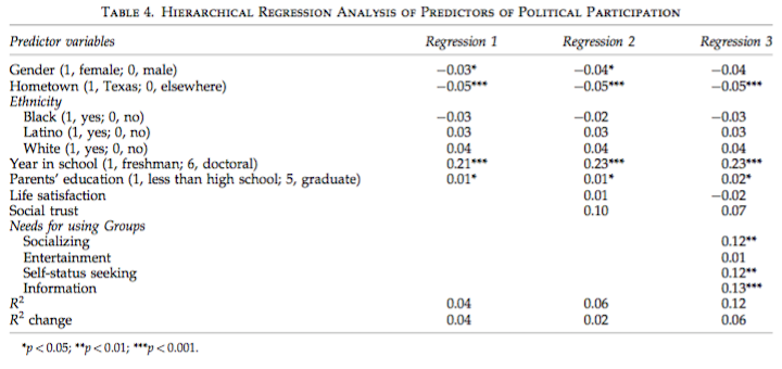
I believe these are standardized beta coefficients (they call them beta in the results section). It doesn't really matter. The interpretation is the same.
The sample consisted of 1715 college students. The researchers wanted to know why college students use Facebook Groups, and how this is related to their involvement in politcal and civic activities. (The table above is relevant to political activities. There is a similar table in the article for civic activities.) For more details, see the article itself.
In the regression analysis, the researchers first entered a block of demographic variables, such as gender (dummy coded), whether or not the student's hometown is in Texas, i.e., in-state student (dummy coded), ethnicity (three dummy coded variables), and two numeric variables that I have issues with, but that's for another time: year in school (coded 1 through 6), and parents' education (coded 1 through 5). When the demographic variables were entered by themselves (Regression 1), gender, hometown, year in school, and parents' education were significant predictors of political participation. If these are standardized betas, then year in school is clearly the most important of these predictors.
From this result, in this sample, who was more involved in political activities, on the average, students from Texas or students from elsewhere?
Interpret the coefficient, assuming it is a standardized beta.
Interpret the coefficient for year in school.
Okay, points off for me. What important restriction on those interpretations did I leave out?
Next, the researchers entered a block of two variables that previous research suggested might be important: life satisfaction and social trust. Neither of these were significant predictors of political participation. The same demographic variables remained significant (Regression 2). Notice that delta R-squared at this step was a mere 0.02, and although the significance of this was not indicated, I think we are safe in assuming that this was not a significant change in R-squared.
Does this mean life satisfaction and social trust have no relationship to political participation?
In the final regression (Regression 3), the researchers entered the four reasons students might be engaging in Facebook Groups use: socializing, entertainment, self-status seeking, and information. Three of these were significant predictors of political participation, and all were about of equal importance: socializing, self-status seeking, and information. The delta R-squared was 0.06 at this step, and that was undoubtedly significant.
Is Regression 3 (by itself) a standard multiple regression (simultaneous regression)?
When all of the predictors are included in the regression analysis, what percentage of the total variability in political participation score is accounted for?
Why so little?
These effects, with the exception of year in school, were small but sometimes turned out to be highly significant due to the very large sample size. Once again, the moral of this story is, if you want to see small effects...???