First, a little review of standard multiple regression.
PART ONE: DATA SUMMARIZATION
According to the so-called self-esteem movement in education (which I suspect you've all been victimized by), a student's self-esteem is critical to his/her school achievement and, therefore, every opportunity should be taken to build the student's sense of self-esteem. Do the data support the role of self- esteem in achievement?
We will attempt to duplicate an analysis in Keith's textbook Multiple Regression and Beyond (1st ed., 2006). Get and summarize the data as follows. It is not available as a text file, so it will have to be read in as a CSV.
> NELS = read.csv("http://ww2.coastal.edu/kingw/psyc480/data/nels.csv")
> dim(NELS)
[1] 1000    5
> summary(NELS)
 std.achieve.score      SES            prev.grades    self.esteem       locus.of.control
 Min.   :28.94     Min.   :-2.41400   Min.   :0.50   Min.   :-2.30000   Min.   :-2.16000
 1st Qu.:43.85     1st Qu.:-0.56300   1st Qu.:2.50   1st Qu.:-0.45000   1st Qu.:-0.36250
 Median :51.03     Median :-0.08650   Median :3.00   Median :-0.06000   Median : 0.07000
 Mean   :50.92     Mean   :-0.03121   Mean   :2.97   Mean   : 0.03973   Mean   : 0.04703
 3rd Qu.:59.04     3rd Qu.: 0.53300   3rd Qu.:3.50   3rd Qu.: 0.52000   3rd Qu.: 0.48000
 Max.   :69.16     Max.   : 1.87400   Max.   :4.00   Max.   : 1.35000   Max.   : 1.43000
 NA's   :77                           NA's   :17     NA's   :59         NA's   :60
NELS stands for National Educational Longitudinal Study. NELS was a study begun in 1988, when a large, nationally representative sample of 8th graders was tested, and then retested again in 10th and 12th grades. These aren't the complete NELS data but 1000 cases chosen, I assume, at random. (Read all about NELS here if you're curious: NELS88.)
The variables are:
1) How many cases (subjects) are there in this dataset? In other words, what
is n?
2) Are there any missing values in any of these variables (yes/no)?
It appears that Keith used SPSS in his analysis. Let's see how close we can come to getting everything (of value) that Keith got from SPSS.
We already have the means, but let's get them again. Since this data frame is all numeric, we can use the apply() function. (Note: For the means, we could also use the colMeans() function, which has a simpler syntax, but it cannot be used to get variances and so forth, so I will stick to apply().)
> apply(NELS, 2, mean)   # the 2 means column means in case you forgot
std.achieve.score               SES       prev.grades       self.esteem  locus.of.control
               NA         -0.031205                NA                NA                NA
Uh oh! What went wrong? Notice in our previous summary that the variables have missing values. When there are missing values, the mean() function in R will fail, because R is smart enough to know that, when there are missing values, there really isn't a mean in the conventional sense. We need to tell R to ignore the missing values by using the appropriate option. Fill in the means. I won't give you check buttons because you can check them against the R output.
> apply(NELS, 2, mean, na.rm=T) # remove missing values first
| std.achieve.score | SES | prev.grades | self.esteem | locus.of.control |
Keith's SPSS output gives these means as 50.9181, -3.1E-02, 2.970, 3.97E-02, and 4.70E-02. Did we get them right?
3) Do these means seem reasonable given the variables we supposedly have
(yes/no)?
Standard deviations can be obtained the same way.
> apply(NELS, 2, sd, na.rm=T)
| std.achieve.score | SES | prev.grades | self.esteem | locus.of.control |
Keith's SPSS output gives these SDs as 9.9415, .77880, .752, .6729, and .6236. Did SPSS get them right?
4) Do they seem right for standardized scores (yes/no)?
Sample sizes are another problem. The na.rm= option does not work with the length() function. We know that we have a thousand cases, and we know how many missing values there are in each variable (above), so we could rely on simple subtraction, but it seems there should be a more elegant way. So I'm going to write a simple function (which I'll explain below) to do it. The function will be placed in your workspace and will remain there until you delete it.
> sampsize = function(X)  sum(!is.na(X))
> apply(NELS, 2, sampsize)
| std.achieve.score | SES | prev.grades | self.esteem | locus.of.control |
These are the values Keith got and which we could have gotten by subtraction. The function works as follows. is.na(X) will go through a variable value by value, checking to see if it's a missing value (NA). If it is, that value will be flagged as TRUE, otherwise it will be flagged as FALSE. When you ask to sum those values, R sums them as if TRUE=1 and FALSE=0. So sum(is.na(X)) will count the number of missing values in a variable. The "!" in the mix means NOT. So !is.na(X) means "is not NA." Then sum() counts the values in the variable that are not NAs. Simple, right?:^)
The next thing Keith got from SPSS was a correlation matrix. The cor() function
in R will also fail if there are missing values, because R wants to know how we
prefer to deal with them. Do we want to use pairwise complete cases? Or do we
want to include only complete observations? That was not clear in the SPSS
output, so I tried it both ways. It turns out SPSS was using only complete
obsevations (i.e, cases with no missing values on any variable).
> cor(NELS, use="complete.obs")   # use="pairwise.complete" is the alternative
                  std.achieve.score       SES prev.grades self.esteem locus.of.control
std.achieve.score         1.0000000 0.4299589   0.4977062   0.1727001        0.2477357
SES                       0.4299589 1.0000000   0.3254019   0.1322685        0.1942161
prev.grades               0.4977062 0.3254019   1.0000000   0.1670206        0.2283377
self.esteem               0.1727001 0.1322685   0.1670206   1.0000000        0.5854103
locus.of.control          0.2477357 0.1942161   0.2283377   0.5854103        1.0000000
SPSS gave Keith these values. (He used different variable names. I changed them to make them a little more comprehensible.) Did SPSS get them right?
          achieve    SES grades esteem    LOC
achieve     1.000
SES         0.430  1.000
grades      0.498  0.325  1.000
esteem      0.173  0.132  0.167  1.000
LOC         0.248  0.194  0.228  0.585  1.000
Note the correlations of the predictors with the achievement scores. The correlation with esteem is the lowest, but it is nevertheless positive and statistically significant. How many cases contributed to this correlation?
5) Do we know how many complete cases there are in these data (yes/no)?
> sum(complete.cases(NELS))
[1] 887
> source("http://ww2.coastal.edu/kingw/psyc480/functions/rcrit.R")   # the r.crit function
> r.crit(df=885)   # remember, for a correlation, df=n-2
      df    alpha   1-tail   2-tail
885.0000   0.0500   0.0553   0.0658
The complete.cases() function works similarly to the is.na() function, except on a case by case basis. It examines each case in the data frame, and if the case is complete (i.e., contains no NAs), then that case is TRUE, otherwise it is FALSE. The sum() function then counts the cases that are TRUE. Thus, the correlations are based on 887 complete cases.
PART TWO: STANDARD MULTIPLE REGRESSION
The next thing Keith got was a standard multiple regression. (He calls it simultaneous regression. Why would he do that?) Here is his SPSS-like output. (Pardon the uneven exposure. I had to take a photo of it under my desk lamp. From pg. 77 of Keith's text.)
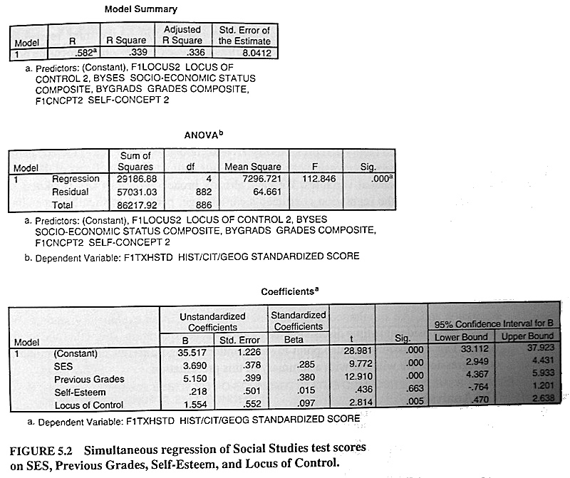
Okay, let's see how much of that we can duplicate. Keith did not include any interaction terms, so we won't either.
> lm.out = lm(std.achieve.score ~ SES + prev.grades + self.esteem + locus.of.control, data=NELS)
> summary(lm.out)

Call:
lm(formula = std.achieve.score ~ SES + prev.grades + self.esteem +
    locus.of.control, data = NELS)

Residuals:
     Min       1Q   Median       3Q      Max
-24.8402  -5.3648   0.2191   5.6748  20.3933

Coefficients:
                 Estimate Std. Error t value Pr(>|t|)
(Intercept)       35.5174     1.2256  28.981   <2e-16 ***
SES                3.6903     0.3776   9.772   <2e-16 ***
prev.grades        5.1502     0.3989  12.910   <2e-16 ***
self.esteem        0.2183     0.5007   0.436    0.663
locus.of.control   1.5538     0.5522   2.814    0.005 **
---
Signif. codes:  0 '***' 0.001 '**' 0.01 '*' 0.05 '.' 0.1 ' ' 1

Residual standard error: 8.041 on 882 degrees of freedom
  (113 observations deleted due to missingness)
Multiple R-squared:  0.3385,	Adjusted R-squared:  0.3355
F-statistic: 112.8 on 4 and 882 DF,  p-value: < 2.2e-16
Okay then, let's see how much of it SPSS got right. Under the Model Summary in Keith's output, the value of R is just the square root of R Square and is really fairly useless, so the first value we want to look at is R Square.
6) What value did we get for that?
It's time to explain Adjusted R-squared. In standard multiple regression, every time you add a new predictor, unless it has no predictive value at all, R-squared will go up. Thus, if you want a higher R-squared, add more predictors! Also, there is a rule of thumb in regression that says you should have at least 10 cases for every predictor you use. Violating that rule will also inflate R-squared. You'll occasionally see in the literature people using a ridiculous number of predictors with very small sample sizes. R-squared doesn't care, but Adjusted R-squared does! Eventually, Adjusted R-squared will start penalizing you for having too many predictors. So while R-squared always goes up when a new predictor is added, Adjusted R-squared might well go down. Keep an eye on Adjusted R-squared as you add predictors to your regression model. If it starts going down, you're overloading your model with predictors.
7) Does our value of Adjusted R-squared agree with Keith's (yes/no)?
8) Now you're going to have to remember something I told you earlier in the
semester. What value did we get for Std Error of the Estimate?
Keith's second table is an ANOVA table. That result is on the bottom line of our output.
9) Does our ANOVA agree with Keith's ANOVA (F, dfs, and p-value the same)?
Keith's output for the ANOVA is a little more elaborate than ours, but if you want the sums of squares and mean squares, here they are.
> anova(lm.out)
Analysis of Variance Table

Response: std.achieve.score
                  Df Sum Sq Mean Sq  F value    Pr(>F)
SES                1  15939 15938.6 246.4953 < 2.2e-16 ***
prev.grades        1  12345 12344.6 190.9127 < 2.2e-16 ***
self.esteem        1    392   391.6   6.0566  0.014045 *
locus.of.control   1    512   512.0   7.9182  0.005003 **
Residuals        882  57031    64.7
---
Signif. codes:  0 '***' 0.001 '**' 0.01 '*' 0.05 '.' 0.1 ' ' 1
113 observations deleted due to missingness
Now our ANOVA output is more elaborate! We have SSes for each of the predictors. If you add them together, you should get SS.Regression in Keith's output. (You'll have to divide that by 4 to get MS.Regression, should you want it. MSes don't add, remember.) Of course, the effects shown in our ANOVA table are not the same effects shown in the lm() output. Why not?
             df        SS       MS      F         p
Regression    4  29186.88  7296.72   112.846  <.001
Residuals   882  57031.03    64.661
Total       886  86217.91
Note: I did print(anova(lm.out), digits=7) to get the table with more decimal places before collapsing. Do the following calculations. What do you get?
| calculate this | value | what is it? | |
| 1 - SS.Residuals / SS.Total | |||
| 1 - MS.Residuals / MS.Total |
Here's a puzzle for you. Why can't we get the ANOVA SS.Total by squaring our SD for std.achieve.score (thus getting the variance) and then multiplying by 886 degrees of freedom (this getting the SS)? Close, but no cigar! Think about it before you click the answer button.
Now for the meat and potatoes of the output, the coefficients.
10) But first, what did we get from R that SPSS did not provide?
11) SPSS puts the coefficients in a column labeled B. Are they the same as R's
coefficients (yes/no)?
12) How about the standard errors for the coefficients, the t-values, and the
p-values? Are they the same (yes/no)?
13) SPSS supplied two things that are not in the R output. What?
> confint(lm.out)
                      2.5 %    97.5 %
(Intercept)      33.1120344 37.922735
SES               2.9491568  4.431499
prev.grades       4.3672598  5.933147
self.esteem      -0.7643607  1.201002
locus.of.control  0.4700688  2.637597
14) Now we have confidence intervals. Are they the same as SPSS's confidence
intervals?
Beta coefficients are going to be tricky, because the SDs we have (and that SPSS supplied) are not calculated from the same cases that were included in the regression, since the regression was calculated only from complete cases. So let's fix that.
> NELS2 = na.omit(NELS)   # omit all cases with missing values
> apply(NELS2, 2, sd)
std.achieve.score               SES       prev.grades       self.esteem  locus.of.control
        9.8646552         0.7630946         0.7283067         0.6661508         0.6147918
15) Now that you can calculate (have calculated!) the standardized beta
coefficients, how are they different from the ones SPSS supplied?
Here's a quick way to do it, by the way.
> SDs = apply(NELS2, 2, sd)   # put the SDs into a vector
> coeffs = lm.out$coef        # put the regression coefficients into a vector
> coeffs * SDs / 9.8646552    # 1st coeff * 1st SD / 9.86; 2nd coeff * 2nd SD / 9.86; etc.
     (Intercept)              SES      prev.grades      self.esteem locus.of.control
     35.51738451       0.28547063       0.38023909       0.01474298       0.09683904
Ignore the value given for the intercept. It's meaningless. We all know the beta coefficient for the intercept is zero, don't we?
16) How would you evaluate the relative "importance" of the predictors?
Notice that the effect of esteem is not significant. How do we reconcile this with the finding above that there is a significant positive correlation between achievement and esteem?
PART THREE: REGRESSION DIAGNOSTICS
Keith doesn't show these for this analysis, but let's do it anyway. Note: I think you can get these in SPSS, but it's a lot more trouble. (Not sure, to be honest.)
> par(mfrow=c(2,2))
> plot(lm.out, 1:4)
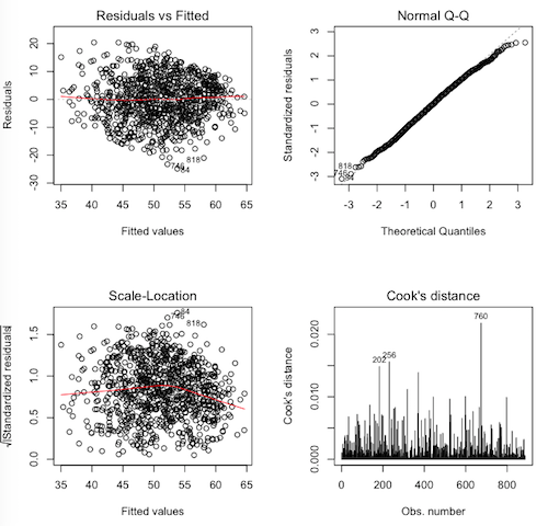
Interpret.
| graph | assumption tested | met or not met | check |
| Residuals vs. Fitted | |||
| Normal Q-Q | |||
| Scale-Location | |||
| Cook's distance |
PART FOUR: HIERARCHICAL REGRESSION
Now that we have reviewed standard multiple regression, and you have a thorough understanding of it, let's move on to hierarchical regression. Keith calls it sequential regression, a name I like, too.
Let's talk a little about what hierarchical regression does that the standard regression does not. I think Keith's exposition on this is so clear that I'm going to essentially paraphrase it, and I'll refer you to his textbook for more. (He covers hierarchical regression only briefly, but it is an excellent summary.)
Standard regression enters all of the predictor variables at once into the regression, and each predictor is treated as if it were entered last. That is, each predictor variable in the regression table above is controlled for all of the other predictors in the table. Another way to say it is, variability in the response that can be attributed to the other predictors is removed before a given predictor is entered. Thus, we can say that the effect of SES is 3.6903 when grades, esteem, and LOC are held constant or are held at their mean values.
The following diagram, which I have redrawn from Keith (Figure 5.7, page 83), shows what this means most clearly.
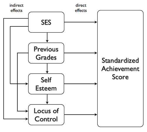
In the little regression universe that we've created for ourselves, the predictors can influence the response potentially over several pathways. For example, SES can have a direct effect on achievement scores, indicated by the arrow that goes straight to the response, but it can also have effects that follow indirect pathways. It can have an effect on locus of control, which then affects achievement scores. It can have an effect on self esteem, which can then act directly on achievement scores, but can also act through locus of control. Following the other arrows around (other than the arrows showing direct effects) will show us how WE THINK each of these predictors might have an indirect effect on achievement scores.
Standard regression reveals only the direct effects of each predictor. Because SES is treated as if it is entered last in a standard regression, all of the indirect effects of SES have already been pruned away, having been handed over to one of the other predictors, before SES gets to attempt to claim variability in the response. Thus, SES is left only with its direct pathway. The other predictors are treated the same way. Standard (or simultaneous) multiple regression shows direct effects ONLY.
However, if SES were entered alone into a regression analysis (as the only predictor, that is), we would get to see its total effect on achievement score, which is its effect through both direct and indirect pathways, because it wouldn't be competing with other predictors for response variability. (It would be the only hog feeding at the trough. AND the hog would be claiming ALL of the variability it is responsible for, direct or mediated, even if it's through mediators we haven't thought of.)
That's what a hierarchical regression does. If SES were entered first into a hierarchical regression, it would get to claim all the response variability it could without having to compete with other predictors. In other words, we wouldn't be seeing just the direct effect of SES on achievement scores, we'd be seeing the total effect. Then when we enter Previous Grades second, we'd get to see its total effect, provided none of that effect goes through SES and, therefore, has already been claimed. (We can't allow any arrows pointing upwards in this diagram. That's not to say they don't exist, but in our model they don't exist. Cause and effect can flow only downward and to the right in our model.) Then we enter Self Esteem third, and we see it's total effect, provided none of that goes through either Previous Grades or SES. Finally, we enter Locus of Control, and since it's the last term in the model, its total effect is the same as its direct effect, because all of the downward pointing arrows that end at LOC have already been stripped away by the predictors entered previously. That's not to say that the effect of LOC isn't mediated somehow or other, but if it is, we haven't yet thought of how and have not included those variables in our little universe.
Is this the way the world really works? Probably not. Models are always simpler than the real world. I'll also remind you once more of what George Box said: "All models are wrong, but some are useful." Have we accounted for all the influences on achievement test scores? Almost certainly not! And if self-esteem is influencing achievement now, in the form of achievement test scores, why wasn't it influencing achievement previously, in the form of previous grades? The self-esteem movement people would probably want to enter self-esteem second in this analysis. Every model can be nitpicked. That's why you get to write a discussion section!
In other words, standard regression reveals direct effects only. In standard multiple regression, all of those downward pointing arrows are stripped away and tossed into the trash can. Why would you want to do that? For the same reason you'd want to do Type III sums of squares in ANOVA. If those other predictors are nothing but confounds, then remove those confounding effects before looking at the effect of any one predictor.
Hierarchical regression, on the other hand, reveals total effects, provided we have entered the predictors in the correct order, AND provided that we have our causal model correct. Those are BIG provideds! Order of entering the predictors is the biggest catch in hierarchical regression. How do we know what order to use? Keith recommends drawing a diagram like the one above. Such a diagram should make it clear in what order the variables should be entered. The diagram should be based on a thorough knowledge of the literature and of these phenomena, not on a whim, some idle speculation, or something that came to you in a dream. If you can't draw such a diagram, then you probably shouldn't be using hierarchical regression.
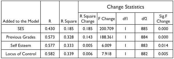
Here are the hierarchical (or sequential as Keith calls it) multiple regression results (Figure 5.3, page 79) as SPSS (I assume) calculated them. The variables were entered one at a time in the order shown in the table.
R is silliness. It's the square root of R Square, and I fully intend to ignore it. R Square is the value of Multiple R-squared at that point in the regression. R Square Change is how much R Square has increased over the preceding step. In other words, it is what we have been calling (and what everyone else calls) delta R-squared. F Change is the F-test on delta R-squared. df1 and df2 should be obvious. Finally, there is a p-value, which allows us to evaluate if the amount of change in R Square due to the entry of that predictor is significant.
Let us recall the ANOVA table we got above.
> print(anova(lm.out), digits=7)   # print() is used to get more significant digits
Analysis of Variance Table

Response: achieve
           Df   Sum Sq   Mean Sq   F value     Pr(>F)
SES         1 15938.64 15938.645 246.49535 < 2.22e-16 ***
grades      1 12344.62 12344.616 190.91274 < 2.22e-16 ***
esteem      1   391.62   391.623   6.05655  0.0140453 *
LOC         1   512.00   512.001   7.91823  0.0050028 **
Residuals 882 57031.03    64.661
---
Signif. codes:  0 '***' 0.001 '**' 0.01 '*' 0.05 '.' 0.1 ' ' 1
We also need to recall the total sum of squares, SS.Total=86217.92. This is a sequential analysis, so shouldn't this be what we're after? Well....
We can get the change in R-squared values by dividing each SS by the total.
> c(15938.64, 12344.62, 391.62, 512.00) / 86217.92
[1] 0.184864585 0.143179283 0.004542211 0.005938441
17) Does this agree with Keith's result (yes/no)?
Of course, the R Square column is just the cumulative sum of those.
> cumsum(c(15938.64, 12344.62, 391.62, 512.00) / 86217.92)
[1] 0.1848646 0.3280439 0.3325861 0.3385245
18) Does this agree with Keith's result (yes/no)?
If you want to be really anal about it, the R column is the square root of those.
Now things appear to go a bit off the rails, however. Notice that our ANOVA table does not give the same tests (except for the last one). Why? The answer is that the ANOVA table tests are done with a common error term, namely, the one shown in the table. There is some disagreement about this. I've seen it done this way in a few other textbooks, but it is not generally considered to be correct. (To be honest, I don't quite understand why. If this were an ANOVA on categorical IVs using Type I sums of squares, this would be considered correct, but in sequential regression with numeric IVs, it is not. Go figure!)
The tests in the SPSS table can be obtained from the ANOVA for any term by pooling all the terms below it in the table with the error term. For example, the test for self.esteem would be:
> ((391.62)/1) / ((512.00+57031.03)/(1+882))   # F value
[1] 6.009424
> pf(6.009424, 1, 883, lower=F)   # p-value
[1] [1] 0.01442249
19) Does this agree with Keith's result (yes/no)?
To much arithmetic for you? Then here's another way to do it in R. Be absolutely certain when you do this to use a version of the data frame from which incomplete cases have been removed! (You'll want your browser window set WIDE at this point!)
> summary(aov(std.achieve.score ~ SES, data=NELS2))   # correct test on SES
             Df Sum Sq Mean Sq F value Pr(>F)
SES           1  15939   15939   200.7 <2e-16 ***
Residuals   885  70279      79
---
Signif. codes:  0 '***' 0.001 '**' 0.01 '*' 0.05 '.' 0.1 ' ' 1

> summary(aov(std.achieve.score ~ SES + prev.grades, data=NELS2))   # correct test on prev.grades
             Df Sum Sq Mean Sq F value Pr(>F)
SES           1  15939   15939   243.2 <2e-16 ***
prev.grades   1  12345   12345   188.4 <2e-16 ***
Residuals   884  57935      66
---
Signif. codes:  0 '***' 0.001 '**' 0.01 '*' 0.05 '.' 0.1 ' ' 1

> summary(aov(std.achieve.score ~ SES + prev.grades + self.esteem, data=NELS2))   # correct test on self.esteem
             Df Sum Sq Mean Sq F value Pr(>F)
SES           1  15939   15939 244.579 <2e-16 ***
prev.grades   1  12345   12345 189.429 <2e-16 ***
self.esteem   1    392     392   6.009 0.0144 *
Residuals   883  57543      65
---
Signif. codes:  0 '***' 0.001 '**' 0.01 '*' 0.05 '.' 0.1 ' ' 1

> summary(aov(std.achieve.score ~ SES + prev.grades + self.esteem + locus.of.control, data=NELS2))   # correct test on locus.of.control
                  Df Sum Sq Mean Sq F value Pr(>F)
SES                1  15939   15939 246.495 <2e-16 ***
prev.grades        1  12345   12345 190.913 <2e-16 ***
self.esteem        1    392     392   6.057  0.014 *
locus.of.control   1    512     512   7.918  0.005 **
Residuals        882  57031      65
---
Signif. codes:  0 '***' 0.001 '**' 0.01 '*' 0.05 '.' 0.1 ' ' 1
20) Why does this work?
R makes you do a little more work to get the answer. In my opinion, this is a good thing. How many of you understood how the tests were done when you looked at the change statistics in the SPSS output? How many of you understand it now that we've done the tests step-by-step in R? Sometimes it's possible to make things too easy. If your software is not engaging your cerebral cortex, I'd say you're using the wrong software!
PART FIVE: BLOCKS OF VARIABLES IN HIERARCHICAL REGRESSION
Variables don't have to be entered one at a time into a hierarchical regression. They can also be entered in blocks. This might happen, for example, if the researcher wanted to enter all psychological variables at one time, or if the researcher was uncertain about the order in which they should be entered. Let's say in the current example we wanted to enter esteem and LOC at the same time.
We can test the effect of entering these two variables as a block like this.
> model.1 = aov(std.achieve.score ~ SES + prev.grades, data=NELS2)
> model.2 = aov(std.achieve.score ~ SES + prev.grades + self.esteem + locus.of.control, data=NELS2)
> anova(model.1, model.2)
Analysis of Variance Table

Model 1: std.achieve.score ~ SES + prev.grades
Model 2: std.achieve.score ~ SES + prev.grades + self.esteem + locus.of.control
  Res.Df   RSS Df Sum of Sq      F    Pr(>F)
1    884 57935
2    882 57031  2    903.62 6.9874 0.0009754 ***
---
Signif. codes:  0 '***' 0.001 '**' 0.01 '*' 0.05 '.' 0.1 ' ' 1
The increase in R-squared can be obtained either by summing the SSes in the original ANOVA table and dividing by the total SS...
> (391.62 + 512.00) / 86217.92
[1] 0.01048065
Or it can be obtained from the residual sums of squares (RSS) in the model comparison. After SES and prev.grades are added, RSS (in other words, SS.Error) is 57935. After the block of variables is added, it is 57031, which means the block has pulled an additional 904 out of SS.Error. That is SS.Block, so delta R-squared due to the block is SS.Block/SS.Total, or...
> 904 / 86217.92
[1] 0.01048506
21) Why is this value different than it was the first time we calculated it?
You didn't really have to do this arithmetic, did you? The SS.Block is given in the model comparison table. Just divide that by SS.Total.
This is in agreement with the SPSS output that is in Figure 5.9 in Keith. So, good, SPSS got it right again!
PART SIX: MEDIATION
What's going on with self-esteem? Based on my profound knowledge and absolutely thorough review of the literature (!), I believe there is an effect of self-esteem on achievement, but I believe it is mediated by locus of control. High self-esteem makes a person feel in control of his/her destiny, and in turn this causes her to excell scholastically. (In truth, I believe this "theory" is a total crock, but let's run with it.) What effects would this mediation have in the correlations and standard regression analysis above?
I propose we conduct the following mediation analysis. (Diagram it in the more conventional "triangle" diagram.)
esteem -> LOC -> achieve, esteem -> achieve
We could test this using just the lm() function, but that requires doing three regressions, and that's annoying. So I've written a function to do it. You can thank me later.
> source("http://ww2.coastal.edu/kingw/psyc480/functions/mediate.R")
Now, if I haven't warned you already, I'm going to warn you now. DO NOT DO MEDIATION ANALYSIS WITH MISSING VALUES IN THE DATA FRAME!!! Thus, we want to be sure to use NELS2 in the mediation analysis. The mediate() function works like this.
> with(NELS2, mediate(x=self.esteem, m=locus.of.control, y=std.achieve.score, diagram=T))
Test of Simple Mediation Effect
            X on M   M on Y    total   direct indirect
statistic 0.540276 3.579580 2.557419 0.623457 1.933962
std.err   0.025152 0.644502 0.490301 0.594812 0.359660
p.value   0.000000 0.000000 0.000000 0.294853 0.000000
Sobel.z       n
   5.38  887.00
Bootstrap Resampling Confidence Intervals for Indirect Effect
***not requested***
Here's the diagram the function produced. (Note: diagram=F is the default.)
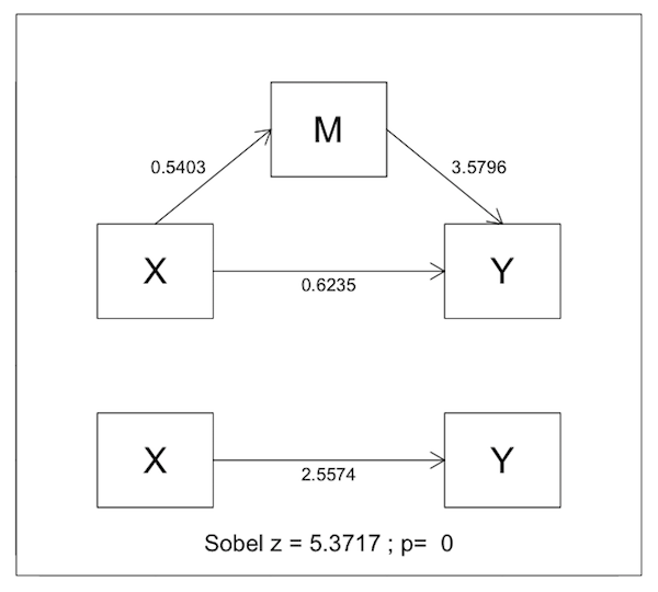
Interpret.
22) What is the magnitude of the total effect of self.esteem on std.achieve.score?
23) Is the total effect statistically significant? Give the p-value.
24) What is the magnitude of the direct effect of self.esteem on std.achieve.score?
25) Is the direct effect statistically significant? Give the p-value.
26) What is the magnitude of the indirect effect of self.esteem on std.achieve.score?
27) Is the indirect effect statistically significant? Give the p-value.
28) Is this complete mediation, partial mediation, or no mediation?
28a) What is percent mediation?
29) Fill in the blank. This result is __________ with the theory that the
effect of self esteem on achievement test scores is mediated by locus of control.
30) What have we forgotten to do?
31) Is there one?
32) Why is that a problem?
PART SEVEN: CONCLUSIONS
What is the effect of self-esteem on scholastic achievement? There are (at least) four conclusions that can be drawn from the above analyses. I'll get you started on each one.
1) There is no
2) There appears to be an
3) Our results are consistent with
4) There may be an
5) In other words, LOC may the effect of self-esteem on scholastic achievement.