a match. These two cards would be removed from the array.
This should work in RStudio Cloud (but I haven't tested it). I'm going to use R. All you need to know FOR NOW is what the output means.
Clear your workspace. Copy everything between the dashed lines and paste it into your R Console. Then press the Enter key.
# --------------------------------------------------------------------------
# clear the workspace
rm(list=ls())
# get a couple data files
file = "http://ww2.coastal.edu/kingw/psyc480/data/matching.txt"
cards = read.table(file=file, header=T, stringsAsFactors=T)
file = "http://ww2.coastal.edu/kingw/psyc480/data/matchinglong.txt"
cards2 = read.table(file=file, header=T, stringsAsFactors=T)
# get the rmsaov.test() function
source("http://ww2.coastal.edu/kingw/psyc480/functions/rmsaov.R")
# create the SS() function
SS = function(X) sum(X^2) - sum(X)^2 / length(X)
# inspect the workspace
ls()
# --------------------------------------------------------------------------
You now have a couple data sets in your workspace, along with the rmsaov.test() function and a custom function to calculate sum of squares.
> ls()
[1] "cards"       "cards2"      "file"        "rmsaov.test" "SS"
The data are from Wes Rowe (Psyc 497 Spring 2009). Wes was in one of my 497 classes, and when he told me he wanted to do something with background music, I probably rolled my eyes. That never works! Not only did it work, but the effect he saw was certainly one I never would have expected!
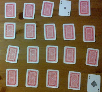
Subjects performed a card matching task under each of three different background music conditions. In this task, an array of playing cards is placed in front of the subject face down. The subject's task is to turn the cards over two at a time and find matching pairs of cards. If the cards don't match, they are turned face down again. If they do match, they are removed from the array. Time required to complete all matches was recorded (in seconds). All subjects were CCU students living in student housing.
A graphic stolen...er, um, borrowed from the Internet showing
a match. These two cards would be removed from the array.
The head() function shows the first several lines of a data frame.
> head(cards, 10)   # first ten rows of data
     X Gender NMTx CMTx IRMTx
1   S1   Male  218  203   161
2   S2   Male  181  196   167
3   S3   Male  158  164   180
4   S4   Male  169  178   151
5   S5 Female  190  182   166
6   S6 Female  141  169   178
7   S7   Male  229  221   196
8   S8 Female  169  156   152
9   S9   Male  208  206   192
10 S10   Male  196  178   173
X is a subject identifier. Gender is gender. NMTx is solving time in a no-music
control condition. CMTx is solving time in a classical music condition. IRMTx is
solving time in an instrumental rap music condition. Long format or wide (short) format?
> head(cards2, 10)   # first ten rows of data
   times gender     music subjects
1    218   Male      none       S1
2    203   Male classical       S1
3    161   Male   instrap       S1
4    181   Male      none       S2
5    196   Male classical       S2
6    167   Male   instrap       S2
7    158   Male      none       S3
8    164   Male classical       S3
9    180   Male   instrap       S3
10   169   Male      none       S4
Long format or wide format?
The "cards" data frame is in wide (short) format. The first column, X, is a subjects identifier. We don't need that in a wide format data frame as each line (row) in the data frame represents all scores from one subject. The second column is subject gender. There was no (obvious) gender effect on any of the three types of background music scores (by t-test, but what kind of effect wouldn't be found this way? ), so we're going to get rid of that variable as well. We will "NULL" them out.
cards$X = NULL
cards$Gender = NULL
head(cards)   # six lines of data is the default
  NMTx CMTx IRMTx
1  218  203   161
2  181  196   167
3  158  164   180
4  169  178   151
5  190  182   166
6  141  169   178
Now the data frame is all numeric with one subject per row and the DV in the columns, perfect for use with the rmsaov.test() function (but we have to remember to make it a matrix first). The three kinds of background music were none (NMTx = no music solving time), classical (CMTx = classical music solving time), and instrumental rap (IRMTx = instrumental rap music solving time). I didn't even know there was such a thing as instrumental rap when Wes did this study, so this was an education for me, too.
The "cards2" data frame is in long format. The existence of the gender column does no harm. The subjects column must be there. The IV is music. The DV is times, which is solving time in seconds. The IV and DV each have their own column in a long format data frame.
> summary(cards2)
     times          gender         music       subjects
 Min.   :141.0   Female:81   classical:52   S1     :  3
 1st Qu.:172.8   Male  :75   instrap  :52   S10    :  3
 Median :185.5               none     :52   S11    :  3
 Mean   :186.6                              S12    :  3
 3rd Qu.:199.0                              S13    :  3
 Max.   :242.0                              S14    :  3
                                            (Other):138
How do we know this summary is from a long format data frame? We know because there is only one summary of the DV. If you were to summarize the wide (short) format data frame (go ahead and try it), you would not get a summary of the DV, you would get a summary of each level of the DV separately. That is, you would have a summary of each music type separately. Because cards2 is a long format data frame, the rmsaov.test() function will not work with it.
How may subjects did Wes test in his study? Be careful! It's tricky!
(Answer: You might be tempted to think 81 females plus 75 males equals 156 subjects. You'd be wrong. Remember, in a long format data frame, each subject has as many rows in the data frame as there are treatments. In this case, there are three treatments, so each subject has three rows. Thus, there are not 156 subjects, but 156/3=52 subjects, and they would be 27 females and 25 males. The repeated measures variable, music, gives that away. Each subject does each type of background music once. Therefore, there are 52 subjects.)
This is the sort of study in which order effects might play a substantial role in the results. Let's look at the means in the wide format data frame using apply().
apply(cards, 2, mean)   # the syntax is (name of data frame, 2, function)
    NMTx     CMTx    IRMTx
188.5577 189.3269 182.0385
Note: The 2 in the apply() syntax causes the means to be calculated down the columns. Replacing that by 1 would calculate the row means. The apply() function cannot be used with the long format data frame. Why not?
Suppose the treatments had been given to every subject in that order: no music, followed by classical music, followed by instrumental rap music. What could account for the effect we're seeing?
It could be an effect of background music type. That was Wes's hypothesis. But it could also be simply an effect of order. Maybe practice made the subjects better at the task, and that's why we see the drop in solving time when the subjects are doing the task for the third time.
What would this kind of screw-up be called? Specifically, type of background music is confounded with order of presentation, because we can't tell which of those variables is actually producing the effect, i.e., the decrease in solving times.
One way to control for this is to randomize the order in which the treatments are given to each subject. A better way is to counterbalance. Wes used a form of counterbalancing called complete counterbalancing, in which every possible order of treatment presentation is used, and subjects are assigned at random to one of those orders, with the caveat that each of the orders occurs an equal number of times. With 3 treatments, the number of possible orders is 6 (=3*2*1).
When counterbalancing is used, we can actually analyze for an order effect by including order as one of the IVs in our analysis. Since order would be a between groups variable, that would make the design a mixed factorial. Take my word for it. There was no order effect. So the order variable will not be analyzed. (It's not even in this version of the data, in case you were looking for it.)
Do we need to look at variances at this point to check the homogeneity of variance assumption?
Normal distribution is also not difficult to check if the data frame is in wide format. We're going to do it graphically, by plotting something called a normal QQ plot. Here are the commands I used to do these plots. You can copy and paste them into R.
par(mfrow=c(1,3))
# a graphics window appears
# at this point I used the mouse to make this window wider than it is tall
# then I drew the plots for each music condition in turn
qqnorm(cards$NMTx, main="NMTx")
qqnorm(cards$CMTx, main="CMTx")
qqnorm(cards$IRMTx, main="IRMTx")
The par() function opened a graphics window and set it so that I could plot one row of three graphs. The qqnorm() function does the plotting. All we have to do is name the variable we want to plot. I got a little fancy and gave each of the graphs a main title as well. Here are the graphs.
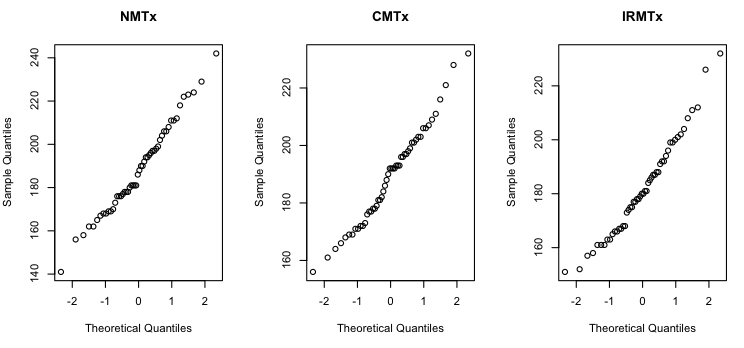
Without going into details, what we want to see on each of those graphs is a straignt line of points going from the lower left corner to the upper right corner. It's not going to be perfectly straight because these are samples and samples are... what? But I'd say they look pretty good. If those lines are bowed, the sample data are skewed. If the bow sags down towards the lower right corner, that's positive skew (skew to the right). If the bow humps up towards the upper left corner, that's negative skew (skew to the left). If that line does weirder stuff, like snakes in an S shape up across the graph, that's an even worse problem than skew! Let's just hope that doesn't happen! In this case, the solving times appear to have a very slight positive skew in all three conditions, but I think we can live with it.
(If you don't remember what a skewed distribution is from your first stat course, Google it!)
Let us analyze.
rmsaov.test(as.matrix(cards))

	Oneway ANOVA with repeated measures

data:  as.matrix(cards)
F = 11.581, df treat = 2, df error = 102, p-value = 2.935e-05

 MS.error  MS.treat  MS.subjs
 72.00289 833.85256 922.62544

Treatment Means
    NMTx     CMTx    IRMTx
188.5577 189.3269 182.0385

HSD.Tukey.95
    3.957991

Compound Symmetry Check (Variance-Covariance Matrix)
          NMTx     CMTx    IRMTx
NMTx  441.7025 313.6180 278.8213
CMTx  313.6180 294.2244 258.1833
IRMTx 278.8213 258.1833 330.7044

Estimated Greenhouse-Geisser Epsilon and Adjusted p-value
    epsilon    p-adjust
0.805520067 0.000127389
I did not want to permanently wreck my data frame by converting it to a matrix forever and all time, so I temporarily converted it to a matrix "on the fly" by using the above method. Let's take a look at the result.
First, we see the ANOVA result, F(2, 102) = 11.581, p < .001. Are those degrees of freedom correct? There were three levels of the music variable, so df=2 is correct for the treatment. There were 52 subjects, so df.subjects=51, which is not shown in the output. There were 3*52=156 scores altogether, so df.total=155, also not shown. That leaves df.error=155-51-2=102. Looks like the computer got it right. Here's another trick for getting error degrees of freedom in these designs. Multiply df.treatment times df.subjects. In this case, that would be 2x51=102.
The p-value is miniscule, so we are convincingly rejecting the null hypothesis. There is at least one significant difference among the mean solving times for the different music types.
Next, the mean squares are given. We can use these to write out a complete ANOVA table, should the desire to do so overwhelm us. And it eventually will, so see if you can do it. The answer will appear below. Some of you have apparently forgotten that MS=SS/df, which means you can get the sums of squares by SS=MS*df. SSes are additive, so SS.total can be had by just adding up SS.treat, SS.subjects, and SS.error. Or, if we have a long format data frame handy...
SS(cards2$times)
[1] 56065.9
Don't forget that SS.total is just the SS of the dependent variable. We could have gotten that from the wide data frame, too, but it would have taken a little more work. For the hopelessly curious...
SS(c(cards$NMTx, cards$CMTx, cards$IRMTx))
[1] 56065.9
Ask if you don't get it (and want to).
The treatment means are next. We've already seen those.
Next comes something called HSD.Tukey.95. That is the Tukey honestly significant difference. Any difference between two means larger than that value is statistically significant by Tukey HSD test. Are there any?
Then we have the variance-covariance matrix. The treatment variances are on the main diagonal of that matrix. In case you forgot, I'll erase everything else so that the main diagonal becomes more obvious.
          NMTx     CMTx    IRMTx
NMTx  441.7025
CMTx           294.2244
IRMTx                   330.7044
What do you think? Have we done okay on homogeneity of variance? Remember, these are sample variances, and samples are noisy, so it would be unreasonable to expect these variances to be the same. But are they close enough that we don't have to worry about the population variances? I'm mildly uncomfortable, but I'm not going to get my shorts in a twist over it.
What about the covariances? Those are the numbers that are off the main diagonal, and they are the same above and below the main diagonal, so we need look at them only once. Covariances do not have to be the same as the variances, and usually won't be, but they should be similar to each other. Are they?
          NMTx     CMTx    IRMTx
NMTx
CMTx  313.6180
IRMTx 278.8213 258.1833
Greenhouse-Geisser Epsilon (GGE) = 0.81, with a best possible value of 1.00 and a worst possible value of...? The adjusted p-value is still very small. So I'd say we've done okay here on the assumptions.
We could have done the analysis as treatment x subjects using the long format data frame as well, but we wouldn't have gotten all the fancy diagnostics. We would have gotten something else though.
aov.out = aov(times ~ subjects + music, data=cards2)   # mind the + sign
summary(aov.out)
             Df Sum Sq Mean Sq F value   Pr(>F)
subjects     51  47054   922.6   12.81  < 2e-16 ***
music         2   1668   833.9   11.58 2.93e-05 ***
Residuals   102   7344    72.0
---
Signif. codes:  0 '***' 0.001 '**' 0.01 '*' 0.05 '.' 0.1 ' ' 1
Is this the same result? By the way, this is the "conventional ANOVA table" that I referred to above, so check yours against this one.
It looks like the same result to me. But this method of analysis gives us an aov.out object, and that allows us to do this.
TukeyHSD(aov.out, which="music")
  Tukey multiple comparisons of means
    95% family-wise confidence level

Fit: aov(formula = times ~ subjects + music, data = cards2)

$music
                        diff        lwr      upr     p adj
instrap-classical -7.2884615 -11.246453 -3.33047 0.0000851
none-classical    -0.7692308  -4.727222  3.18876 0.8890419
none-instrap       6.5192308   2.561240 10.47722 0.0004724
What have we done? What is your interpretation of that? You can reconstruct this table from the rmsaov.test() output using the means and the value for HSD.Tukey.95 (except for the p-values). Can you figure it out? Here is a quick summary of how to do it.
Okay, now for a hard question. When we threw out the gender variable, what did we throw out along with it? Think about it a minute. I said none of the three music types showed a gender effect. Here is one of those tests from the wide (short) format data frame. Too late to do this now, after we've nulled out the Gender column, but I did it before we did that.
> t.test(IRMTx ~ Gender, data=cards, var.eq=T)   # you can't do this now

	Two Sample t-test

data:  IRMTx by Gender
t = 0.029644, df = 50, p-value = 0.9765
alternative hypothesis: true difference in means is not equal to 0
95 percent confidence interval:
 -10.08773  10.38995
sample estimates:
mean in group Female   mean in group Male
            182.1111             181.9600
The other two p-values were both 0.2. So what have we lost by tossing out that gender variable?
Got it yet?
============================================================================
What follows is the analysis of a mixed factorial design, with music as the
within subjects variable and gender as the between groups variable. You do
NOT need to know how to do this at tis time. I'm just making a point. When we
throw out a variable, we lose any chance of seeing an effect of that variable.
We still have the gender variable in the long format data frame, so...
============================================================================
aov.mixed = aov(times ~ gender * music + Error(subjects/music),data=cards2)
summary(aov.mixed)

Error: subjects
          Df Sum Sq Mean Sq F value Pr(>F)
gender     1    841   840.6   0.909  0.345
Residuals 50  46213   924.3

Error: subjects:music
              Df Sum Sq Mean Sq F value   Pr(>F)
music          2   1668   833.9  12.107 1.96e-05 ***
gender:music   2    457   228.5   3.318   0.0403 *
Residuals    100   6887    68.9
---
Signif. codes:  0 '***' 0.001 '**' 0.01 '*' 0.05 '.' 0.1 ' ' 1
How about now?
When we threw out gender, we lost the possibility of seeing an interaction between music and gender. And lookie there! That interaction is significant, too. It looks like the effect of music type is different for females vs. males. Let's see if we can figure out how.
with(cards2, tapply(times, music, mean))
classical   instrap      none
 189.3269  182.0385  188.5577
There are the overall means from the long format data frame. We've seen those. What we need are the means for males and females separately.
> with(cards2, tapply(times, list(gender,music), mean))
       classical  instrap     none
Female  186.2222 182.1111 184.8889
Male    192.6800 181.9600 192.5200
The point you should remember is that, to see the interaction, we need a table of cell means that looks like this, however you get it.
         Mean Solving Times (sec)
          none    classical  instrap
Male     192.52    192.68    181.96
Female   184.89    186.22    182.11
Here's a preliminary question. Overall, who did better, men or women?
Now can you describe the interaction? It looks like women performed well regardless of the type of background music. In fact, if you tested the simple effect, it would not be significant for women. The men only did as well as the women on instrumental rap. They were 6-8 seconds worse in the other two conditions (and that simple effect is significant).
Now that's an interesting effect! Why would that happen?
Here's another very similar analysis, also from a Psyc 497 project. I'll just show the steps in the analysis. Can you explain what's being done and what is being found?
#--------------------copy and paste these lines to follow in R--------------------
rm(list=ls())   # clear workspace (or use the menu)
# read in wide format version of the data frame (only available in csv)
file = "http://ww2.coastal.edu/kingw/psyc480/data/rtcolor.csv"
RT = read.csv(file=file, header=T, stringsAsFactors=T)
# summarize
summary(RT)
#--------------------------------------------------------------------------------
      red             white             blue            green
 Min.   :0.4770   Min.   :0.4560   Min.   :0.4500   Min.   :0.4000
 1st Qu.:0.6085   1st Qu.:0.6015   1st Qu.:0.5760   1st Qu.:0.5455
 Median :0.6990   Median :0.6645   Median :0.6405   Median :0.6045
 Mean   :0.6974   Mean   :0.6608   Mean   :0.6502   Mean   :0.6231
 3rd Qu.:0.7598   3rd Qu.:0.7332   3rd Qu.:0.7250   3rd Qu.:0.6893
 Max.   :0.9530   Max.   :0.8920   Max.   :0.9380   Max.   :0.8870
Here is a description of the data.
Data are from Josh Weiner PSYC 497 Fall 2009. He did a reaction time experiment in which he tested each subject for 5 trials on each of four different colored light stimuli. Recorded reaction time is the mean of those 5 trials for each color by subject. It's a wide format data frame, so each row is a subject and contains all four scores for that subject. There are no IV and DV columns as there would be in a long format data frame.
> head(RT)
    red white  blue green
1 0.662 0.672 0.665 0.602
2 0.695 0.728 0.608 0.670
3 0.659 0.640 0.725 0.673
4 0.806 0.761 0.764 0.785
5 0.517 0.536 0.507 0.400
6 0.744 0.828 0.848 0.766
What is the potential confound here? Josh had to be very careful to
control for something. What? Okay, order. He did that by randomizing. But
there is something else, too.
> apply(RT, 2, mean)
red white blue green
0.6973913 0.6608261 0.6502391 0.6231304
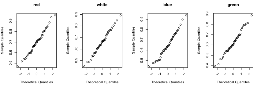
> par(mfrow=c(1,4))
> qqnorm(RT$red, main="red")
> qqnorm(RT$white, main="white")
> qqnorm(RT$blue, main="blue")
> qqnorm(RT$green, main="green")
> source("http://ww2.coastal.edu/kingw/psyc480/functions/rmsaov.R")
> rmsaov.test(as.matrix(RT))

	Oneway ANOVA with repeated measures

data:  as.matrix(RT)
F = 18.92, df treat = 3, df error = 135, p-value = 2.653e-10

   MS.error    MS.treat    MS.subjs
0.002298121 0.043481295 0.040506595

Treatment Means
      red     white      blue     green
0.6973913 0.6608261 0.6502391 0.6231304

HSD.Tukey.95
  0.02600257

Compound Symmetry Check (Variance-Covariance Matrix)
              red       white       blue       green
red   0.012013799 0.008655581 0.01060839 0.009776370
white 0.008655581 0.010172814 0.00892922 0.008354757
blue  0.010608393 0.008929220 0.01324241 0.010988390
green 0.009776370 0.008354757 0.01098839 0.011971938

Estimated Greenhouse-Geisser Epsilon and Adjusted p-value
     epsilon     p-adjust
9.292197e-01 9.976223e-10
I hope you remember how scientific notation works!
Here is a Tukey HSD test from an ANOVA on the long format data frame, which I happen to have. (We didn't download it.) Can you reproduce the table (except for the p-values) from the result above? What is being found here?
> TukeyHSD(aov.out, which="Color")
  Tukey multiple comparisons of means
    95% family-wise confidence level

Fit: aov(formula = RT ~ Color + factor(Subject), data = RT2)

$Color
                   diff         lwr          upr     p adj
green-blue  -0.02710870 -0.05311127 -0.001106125 0.0374772
red-blue     0.04715217  0.02114960  0.073154745 0.0000347
white-blue   0.01058696 -0.01541561  0.036589528 0.7148841
red-green    0.07426087  0.04825830  0.100263441 0.0000000
white-green  0.03769565  0.01169308  0.063698223 0.0013701
white-red   -0.03656522 -0.06256779 -0.010562646 0.0020382
1) Sleep Drugs.
The data are from A.R. Cushny & A.R. Peebles (1905). The action of optical isomers. II. Hyoscines, Journal of Physiology, v.32, pgs.501-510. The data come from a table in that article. The researchers were testing the ability of three hypnotic drugs to produce sleep in people with varying degrees of insomnia. The DV is sleep time in hours. Each patient was measured several times with each drug, and the sleep times are averages of those trials. The object, of course, is to find if the drugs differ in effectiveness. (Note for future psychopharmacology students: L-Hydroscyamine is also called L-atropine. It is the chemical precursor of Hyoscine, which is also called scopolamine, at one time an ingredient in certain cold medicines, but since removed as it is considered too dangerous. Both are muscarinic acetylcholine antagonists.) Historical note: these data were used by Wm. Gosset, aka A.Student, in his development of the t-test.
Copy and paste the following:
# -----------------------------------------------------------------------------
rm(list=ls())
SD = read.csv("http://ww2.coastal.edu/kingw/psyc480/data/sleepdrugs.csv")
SD2 = read.csv("http://ww2.coastal.edu/kingw/psyc480/data/sleepdrugslong.csv")
source("http://ww2.coastal.edu/kingw/psyc480/functions/rmsaov.R")
SS = function(X) sum(X^2) - sum(X)^2 / length(X)
ls()
# -----------------------------------------------------------------------------
Answer: F = 10.277, df treat = 3, df error = 27, p-value = 0.0001096
2) Base Running
Hollander & Wolfe (1973), p.140ff. Comparison of three methods ("round out", "narrow angle", and "wide angle") for rounding first base. For each of 22 players and the three methods, the average time of two runs from a point on the first base line 35ft from home plate to a point 15ft short of second base is recorded. (Times are in seconds.) The obvious question is, is one method better than the others, and if so, by how much?
Copy and paste the following:
# -----------------------------------------------------------------------------
rm(list=ls())
BR = read.csv("http://ww2.coastal.edu/kingw/psyc480/data/baserunning.csv")
BR2 = read.csv("http://ww2.coastal.edu/kingw/psyc480/data/baserunlong.csv")
source("http://ww2.coastal.edu/kingw/psyc480/functions/rmsaov.R")
SS = function(X) sum(X^2) - sum(X)^2 / length(X)
ls()
# -----------------------------------------------------------------------------
Answer: F = 6.2883, df treat = 2, df error = 42, p-value = 0.004084
The End