(Set your browser window fairly wide for this one, perhaps full screen.)
This is a classic problem in multiple regression, and it's going to require you to do something hard. It's going to require you to think! If you put some time in on this problem, you will learn a lot, not only about multiple regression, but about statistics. Ready? Set? Go!
Scottish Hill Races are long distance foot races in which the runners have to run up a hill. The dataset contains three variables: dist, which is how long the race is in miles; climb, which is how high the hill is the runners have to climb in feet; and time, which is the record time for the race in minutes. We are going to try to create a regression model that predicts time from dist and climb.
Some things you may what to think about (and think about them before you read my answers):
Here is a hard lesson in statistics. Somebody's got to enter the data! Here are the data. The name of the race is in the row names.
                 dist climb    time
Greenmantle       2.5   650  16.083
Carnethy          6.0  2500  48.350
Craig Dunain      6.0   900  33.650
Ben Rha           7.5   800  45.600
Ben Lomond        8.0  3070  62.267
Goatfell          8.0  2866  73.217
Bens of Jura     16.0  7500 204.617
Cairnpapple       6.0   800  36.367
Scolty            5.0   800  29.750
Traprain          6.0   650  39.750
Lairig Ghru      28.0  2100 192.667
Dollar            5.0  2000  43.050
Lomonds           9.5  2200  65.000
Cairn Table       6.0   500  44.133
Eildon Two        4.5  1500  26.933
Cairngorm        10.0  3000  72.250
Seven Hills      14.0  2200  98.417
Knock Hill        3.0   350  78.650
Black Hill        4.5  1000  17.417
Creag Beag        5.5   600  32.567
Kildcon Hill      3.0   300  15.950
Meall Ant-Suidhe  3.5  1500  27.900
Half Ben Nevis    6.0  2200  47.633
Cow Hill          2.0   900  17.933
N Berwick Law     3.0   600  18.683
Creag Dubh        4.0  2000  26.217
Burnswark         6.0   800  34.433
Largo Law         5.0   950  28.567
Criffel           6.5  1750  50.500
Acmony            5.0   500  20.950
Ben Nevis        10.0  4400  85.583
Knockfarrel       6.0   600  32.383
Two Breweries    18.0  5200 170.250
Cockleroi         4.5   850  28.100
Moffat Chase     20.0  5000 159.833
Who's going to enter it? Hint: not me! Let me ask you another question. It's not a lot of data, just 35 cases of 3 variables, but do you think you could enter it without making a typing mistake? What if the data were not so neatly typed out for you but were handwritten? What if whoever wrote it had poor handwriting? Take a close look at the data. Do you see anything there that looks like it might be a typo? No? Really? Take another look at the race called Knock Hill.
A further note on the data: these data are old, from the 1970s, I believe. There are updated data at the Scottish Hill Racing website. Or at least there used to be. The website appears to have changed. We're not going to worry about it.
Get the data as follows. It's a built-in dataset, so lucky you!
> data(hills, package="MASS")
> head(hills)   # first six rows; head(hills,10) will show you ten rows
             dist climb   time
Greenmantle   2.5   650 16.083
Carnethy      6.0  2500 48.350
Craig Dunain  6.0   900 33.650
Ben Rha       7.5   800 45.600
Ben Lomond    8.0  3070 62.267
Goatfell      8.0  2866 73.217

> dim(hills)   # rows by columns (you remembered that, didn't you?)
[1] 35  3

> summary(hills)
      dist            climb           time
 Min.   : 2.000   Min.   : 300   Min.   : 15.95
 1st Qu.: 4.500   1st Qu.: 725   1st Qu.: 28.00
 Median : 6.000   Median :1000   Median : 39.75
 Mean   : 7.529   Mean   :1815   Mean   : 57.88
 3rd Qu.: 8.000   3rd Qu.:2200   3rd Qu.: 68.62
 Max.   :28.000   Max.   :7500   Max.   :204.62

> apply(hills, MARGIN=2, FUN=sd)   # the FUN we're having here is getting the SDs
       dist       climb        time
   5.523936 1619.150536   50.334972
The name of the race is in the row names, "dist" is the distance in miles that has to be run, "climb" is the height of the hill in feet that must be climbed to reach the finish line, and "time" is the record winning time for the race in minutes. The obvious question of interest is, how is time determined by dist and climb?
The data frame is all numeric, and there are no missing values, so cor() should give us the correlation matrix without too much fuss.
> cor(hills)
           dist     climb      time
dist  1.0000000 0.6523461 0.9195892
climb 0.6523461 1.0000000 0.8052392
time  0.9195892 0.8052392 1.0000000
Question. What is the correlation between dist and time? (You can
round off to three decimal places if you want to. I'm going to!)
Question. What is the correlation between time and climb?
Question. These correlations seem pretty high. Is that a good thing
or a bad thing?
Question. The correlation between dist and climb is 0.652. (Or am I
lying?) Is that a good thing or a bad thing?
How bad is it? There is a statistic called the "variance inflation factor" or VIF (you just wrote that down, right?) that tells you. When there are only two predictors, VIF is easy to calculate. It's:
VIF = 1 / (1 - r^2)
where r is the Pearson correlation between the two predictors.
Variance inflation makes it difficult to find significant effects in a regression analysis. When VIF reaches 5 or more, we should start to worry. If it reaches 10 or more, then we have a very serious problem with variance inflation. VIF=1 means there is no variance inflation. (Note: there is an optional R package at CRAN called "car" that has a VIF function. In my opinion, "car" should be part of the base installation, but then no one has asked for my opinion. We can't install it in the lab, so we'll live without it.)
Question. What is VIF in this case?
Next, we'll look at the scatterplots. The two interesting ones are in the bottom row of the scatterplot matrix, because those are the ones that have the response on the vertical axis.
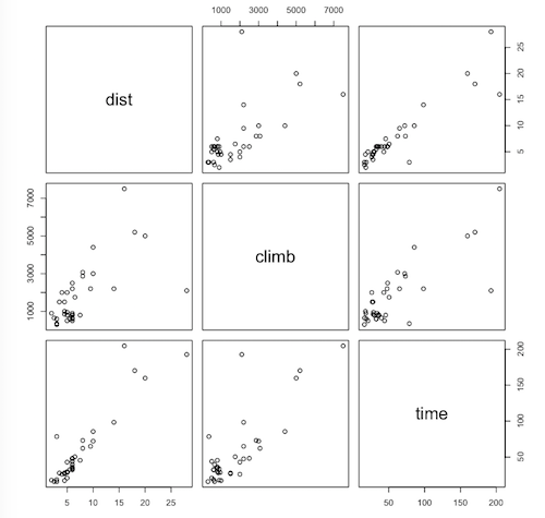
> pairs(hills)
Question. How would you describe the relationship between time and
dist?
Question. Do you see any indication of nonlinearity in the relationship
between time and climb (yes/no/maybe)?
If there is nonlinearity, we're going to ignore it and go ahead and fit a linear model, time ~ dist + climb. (In any event, the nonlinearity does not appear to be serious.)
Question. Are there any obvious outlying points on the time vs. climb
scatterplot?
Now for the regression.
> lm.hills = lm(time ~ dist + climb, data=hills)
> summary(lm.hills)
The output appears below the scatterplot matrix.
Call:
lm(formula = time ~ dist + climb, data = hills)

Residuals:
    Min      1Q  Median      3Q     Max
-16.215  -7.129  -1.186   2.371  65.121

Coefficients:
             Estimate Std. Error t value Pr(>|t|)
(Intercept) -8.992039   4.302734  -2.090   0.0447 *
dist         6.217956   0.601148  10.343 9.86e-12 ***
climb        0.011048   0.002051   5.387 6.45e-06 ***
---
Signif. codes:  0 ‘***’ 0.001 ‘**’ 0.01 ‘*’ 0.05 ‘.’ 0.1 ‘ ’ 1

Residual standard error: 14.68 on 32 degrees of freedom
Multiple R-squared:  0.9191,	Adjusted R-squared:  0.914
F-statistic: 181.7 on 2 and 32 DF,  p-value: < 2.2e-16
Question. There are several disturbing things in this output. Reading
from top to bottom, what's the first one you see?
It's a foot race. We should be able to predict the finishing time pretty accurately from the dist alone. If you did the recordtimes.txt exercise, you know we're very good at predicting record times from distance. How could we have missed one by 65 minutes?
Question. Here's the next thing that struck me as odd from this result.
Examine the intercept in the table of regression coefficients. Do you find it
in any way disturbing that the intercept is significantly different from zero
(yes/no/maybe)?
What should the intercept be? Think about it. What is the intercept? The intercept is the prediction when all the predictors are set to zero. The prediction for a foot race of zero distance and zero climb should be zero minutes, wouldn't you say? It should take you no time at all to run nowhere! Instead, our model is telling us, if we stand on the starting the line of a zero-distance, zero-climb foot race, and the starter fires the starting pistol, we will be instantly 9 minutes younger! It seems we've invented a statistical time machine. (Just kidding, but hopefully you get my point.)
Question. It would be unrealistic to expect the intercept from
sample data to be exactly zero. Why?
If you're still missing that one, go directly to jail. Do not pass Go. Do not collect $200. But at least we might expect it not to be significantly different from 0. It's possible in a regression model to force the intercept to be zero, but before we do something so drastic, we should try to figure out what's going wrong with this model.
Question. I have another problem with the model. For a race of 0
climb, how long does it take to run each mile of the race according to this
model?
This is not me out there running these races. These are highly trained athletes. 6 minutes and 13 seconds seems a little slow for a mile.
Question. Yeah, but they're running up a hill. Couldn't that explain
it?
The validity of our model depends upon having met certain underlying assumptions of the procedure. We will now check those.
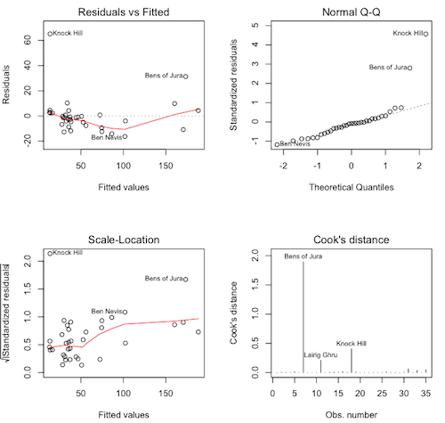
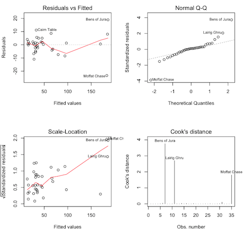
# close the graphics window first, if it's open
> par(mfrow=c(2,2))
> plot(lm.hills, 1:4)
Question. What are these graphs called again?
Question. These are not pretty, but they are also not the worst I've
ever seen. What do we see in the upper left graph?
Question. What about the upper right graph?
Question. What about the lower left graph?
Question. What is the largest Cook's distance (approximately)?
Question. Is that a problem?
Let's look at the three flagged points on the Cook's distance plot.
> hills[c("Bens of Jura","Lairig Ghru","Knock Hill"), ]
             dist climb    time
Bens of Jura   16  7500 204.617
Lairig Ghru    28  2100 192.667
Knock Hill      3   350  78.650
Question. What's up with Bens of Jura? What makes it stand out from
the other races? (You may want to look at the summary again.)
Question. What's up with Lairig Ghru?
It appears that our model may be breaking down for the extreme races. It happens. But what about Knock Hill. There is nothing extreme about Knock Hill. It's a short race and not much of a climb, one of the lowest, in fact. Yet the record time is over 78 minutes. Seriously, I'm not nearly in as good a shape as I used to be, but I could walk three miles in 78 minutes, even if I had to carry a birthday cake! What do you think happened here? The concensus is that this is a recording error and that the correct record time was 18.65 minutes.
Let's change this value. First, we'll make a backup. If you have attached the data frame, detach it before you do this. NEVER modify an attached data frame!
hills.bak = hills   # make a backup, better safe than sorry!
hills["Knock Hill","time"] = 18.65
You could now redo this entire analysis and what you'd discover is this "correction" makes everything worse. The intercept is now -12.942, the coefficient for "dist" is now 6.346, the residuals plot indicates even more of a problem with nonlinearity, the scale-location plot while not bad is also not as good as it was, and Bens of Jura now has a Cook's distance over 4. This shouldn't be happening. This is a fairly simple physical phenomenon. We should be getting a better result than this. What are we missing?
Go back to the questions at the top of this exercise and think some more about question 5. If you can get this, you can count yourself as being very clever.
Scroll down past the image when you're ready for the answer.

When things go screwy like this, it often means there is an effect we are leaving out that is important. There is only one possible such effect in this case, and that is the interaction between the two predictors. Let's see what happens if we include it. In regression analysis, an interaction effect is often referred to as a moderator effect. I'll explain why below.
With two numeric variables predicting a third numeric (response) variable, if there is no interaction, we get a regression surface or plane in three-dimensional space instead of a simple regression line. The actual data points may not, and probably will not, actually fall on this plane, just as they don't fall on the regression line in simple regression. The distance of a data point above or below the plane is called the residual for that data point.
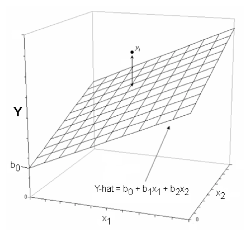
You can think of it this way. In the graph at left, there are two predictors, X1 and X2, and a response, Y. The general form of the regression equation is shown on the "floor" of the graph. The coefficient b0 shows where the plane cuts the Y-axis, while b1 gives the slope of the plane along the X1 axis, and b2 gives the slope along the X2 axis. For each value of X2, there is a different regression line for X1. All those regression lines have the same slope but they have different intercepts. If you exchange X1 and X2 in that last sentence, you'll also have a true statement.
Let's take the (uncorrected) hills result as an example. The regression equation is:
time.hat = -8.992 + 6.218 * dist + 0.0110 * climb
If we set climb = 0, the equation becomes:
time.hat = -8.992 + 6.218 * dist + 0.0110 * 0
         = -8.992 + 6.218 * dist
If we set climb=1000, the equation becomes:
time.hat = -8.992 + 6.218 * dist + 0.0110 * 1000
         =  2.008 + 6.218 * dist
And if we set climb = 2000, the equation becomes:
time.hat = -8.992 + 6.218 * dist + 0.0110 * 2000
         = 13.008 + 6.218 * dist
The slope stays the same but the intercept changes. We could play the same game setting "dist" equal to various values, but that should be obvious by now.
If there is no effect of either X1 or X2 on Y, then the plane will be horizontal at Y=mean(Y). If there is an effect of X1 but not of X2, the plane will be tilted (sloped) in the direction of the X1 axis but not in the direction of the X2 axis. Likewise, if there is an effect of X2 but not of X1, the plane will be tilted in the direction of the X2 axis but not in the direction of the X1 axis. If there is an additive effect of X1 and X2 (as depicted in the figure), then the plane will be tilted in both directions, as if it were standing on one of its corners.
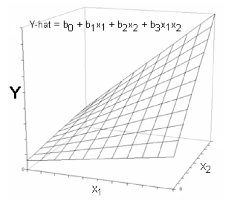
Now let's see what happens if there is an interaction. In regression analysis, an interaction is usually modeled by adding a term in which the predictors are multiplied.
The existence of an interaction causes the plane to become twisted. Along the X1 axis the plane is more tilted at some places than at others. Notice at the low end of the X1 axis the plane is almost horizontal in the X2 direction, while at the high end of the X1 axis the plane is quite sloped. And now, reread the last sentence and interchange X1 and X2. Mathematically speaking, the plane has different slopes in the X2 direction at different values of X1, and different slopes in the X1 direction at different values of X2.
Looked at another way, at low values of X1, X2 has almost no effect on Y. At high values of X1, X2 has a strong effect on Y. Similarly, at low values of X2, X1 has only a slight effect on Y, while at high values of X2, X1 has quite a dramatic effect on Y. Thus, the effect of X1 on Y is moderated by the presence of X2. (We might say vice versa, as well, although in moderator analysis, one of the variables is usually designated at the moderator of the other.) That's why it's called a moderation effect. One variable moderates (or modifies or changes) the effect of the other variable.
Notice that this regression surface is not "bowed" or curved in any way. At any given value of X2, the effect of X1 is still linear, and vice versa.
Now you know I'm not going to all the trouble to explain that unless there actually is an interaction in the hills data. So let's see it. I'll use the corrected data this time.
> lm.hills = lm(time ~ dist * climb, data=hills)   # asterisk means test the interaction
> summary(lm.hills)

Call:
lm(formula = time ~ dist * climb, data = hills)

Residuals:
     Min       1Q   Median       3Q      Max
-23.3078  -2.8309   0.7048   2.2312  18.9270

Coefficients:
              Estimate Std. Error t value Pr(>|t|)
(Intercept) -0.3532285  3.9121887  -0.090 0.928638
dist         4.9290166  0.4750168  10.377 1.32e-11 ***
climb        0.0035217  0.0023686   1.487 0.147156
dist:climb   0.0006731  0.0001746   3.856 0.000545 ***
---
Signif. codes:  0 ‘***’ 0.001 ‘**’ 0.01 ‘*’ 0.05 ‘.’ 0.1 ‘ ’ 1

Residual standard error: 7.35 on 31 degrees of freedom
Multiple R-squared:  0.9806,	Adjusted R-squared:  0.9787
F-statistic: 521.1 on 3 and 31 DF,  p-value: < 2.2e-16
Notice the benefits we've achieved by adding the interaction term. The intercept is now quite close to zero, as would be expected. The effect of "dist" is now much closer to the time we would expect it to take a trained athlete to run a mile. Also, look what happened to R-squared. We are now explaining over 98% of the variability in "time" using just these two predictors.
The regression equation would be (fill in the coefficients to 4 nonzero decimal places):
time.hat = + * dist + * climb + * dist * climbLet's see what happens when we set climb equal to various values. We'll start with climb=0.
time.hat = -0.3532 + 4.9290 * dist + 0.003522 * 0 + 0.0006731 * dist * 0Now we'll do climb=1000.
time.hat = -0.3532 + 4.9290 * dist + 0.003522 * 1000 + 0.0006731 * dist * 1000The intercept has changed, as it did when there was no interaction, but the slope of "dist" has also changed. At climb=0, the effect of "dist" was 4.9290 minutes per mile. At climb=1000 it's taking our trained athletes longer to run each mile, 5.6021 minutes per mile. That's the signature of an interaction. Changing the value of one variable changes the effect of the other variable. It's not so different than it was in ANOVA. In ANOVA we went from level to level of one variable and watched the simple effect of the other variable change. Here we don't have levels, we have numbers, because our variables are numeric.
Now calculate the changes that would occur in the interacept and slope of "dist" if we set climb=2000. I'll get you started. All you have to do is complete the multiplications and combine terms.
time.hat = -0.3532 + 4.9290 * dist + 0.003522 * 2000 + 0.0006731 * dist * 2000
Question. At climb=2000, the new intercept would be:
Question. At climb=2000, the new effect (coefficient) of "dist" would be:
Question. If every race had a climb of 2000 feet, what would the
regression equation be for time on distance?
Has including an interaction term improved our regression diagnostics at all. Let's take a look.
> plot(lm.hills, 1:4)
The regression diagnostics are still a little messy, and that appears to be due to some outliers or influential cases. Bens of Jura has a Cook's D of nearly 4, and Lairig Ghru has a Cook's D of almost 3. In addition Moffit Chase now has a large Cook's distance. Let's look at that one.
> hills["Moffat Chase",]
               dist climb    time
Moffat Chase   20.0  5000 159.833
Also an extreme race. Let's look at the residuals for these outliers.
> lm.hills$residuals[c("Bens of Jura","Lairig Ghru","Moffat Chase")]
Bens of Jura  Lairig Ghru Moffat Chase
   18.927036     8.036745   -23.307768
I'm a little puzzled by this. Can you figure out why? Bens of Jura has the largest positive residual.
Question. Does that mean the prediction for Bens of Jura is too high
or too low?
That's not what puzzles me. If Bens is an extreme race, and the model breaks down for extreme races (because extreme races are harder than the model predicts), we might expect the extreme races to take longer to run than the model predicts. But Moffat Chase has the largest negative residual, meaning the prediction for Moffat is 23.3 minutes TOO HIGH! Moffat is easier than the model predicts. How do we explain that?
Oh! You're waiting for an answer from me? I don't know! Look at the race Two Breweries. That's an 18 mile race with a 5200 foot climb, similar to Moffat Chase. Yet, the residual for Two Breweries is 0.57. R-squared for this model is better than 98%, but there is still something missing. This is where you make some statement in your discussion section about "further research."
If you want to contemplate it, you can see all the residuals sorted in order from most negative to most positive by doing this.
> sort(lm.hills$residuals)
Or you can add the residuals as a column in the data frame like this.
> hills$residuals = lm.hills$residuals
> hills
You can also see the predicted values from the model like this.
> lm.hills$fitted
Happy hunting!
Meaning of Interactions. The coefficient of the interaction term tells us how the interaction works. In the hills analysis, that coefficient is 0.0006731, which tells us that every increase in climb of 1 foot increases the effect of "dist" by 0.0006731 minutes per mile, and likewise, every increase in distance of 1 mile increases the effect of climb by 0.0006731 minutes per foot. The coefficient is positive, so increasing the value of one of the variables by 1 unit increases the effect of the other variable by an amount equal to the coefficient.
1) What do you get from the hill racing model (use the last one with the
interaction, although it wouldn't make any difference) if you do this?
> cor(lm.hills$fitted, hills$time)^2
[1] 0.980557
2) Now I can just tell you're itching for a problem to practice with. Look at Parris Claytor's loneliness data.
# loneliness.txt
# These data are from a Psyc 497 project (Parris Claytor, Fall 2011).
# The subjects were given three tests, one of embarrassability ("embarrass"),
# one of sense of emotional isolation ("emotiso"), and one of sense of social
# isolation ("socialiso"). One case was deleted (by me) because of missing
# values on all variables. Higher values on these variables mean more.

> file = "http://ww2.coastal.edu/kingw/psyc480/data/loneliness.txt"
> lone = read.table(header=T, file=file)
> summary(lone)
   embarrass         emotiso        socialiso
 Min.   : 32.00   Min.   : 0.00   Min.   : 0
 1st Qu.: 52.75   1st Qu.: 5.75   1st Qu.: 2
 Median : 65.00   Median :11.00   Median : 6
 Mean   : 64.90   Mean   :12.07   Mean   : 7
 3rd Qu.: 76.25   3rd Qu.:16.00   3rd Qu.:10
 Max.   :111.00   Max.   :40.00   Max.   :31
3) If you do a standard multiple regression with "emotiso" ("loneliness") as the response, you will discover a significant interaction. Can you write a regression equation that incorporates the interaction term? Can you describe how the interaction works? This one is very interesting. We'll have reason to look at these data again later.
Also, look at the bodyfat.txt data again. Can you explain this?
Call:
lm(formula = fat ~ weight * abdom, data = bfat)

Residuals:
     Min       1Q   Median       3Q      Max
-11.2566  -3.1276  -0.1029   2.9699  10.2832

Coefficients:
               Estimate Std. Error t value Pr(>|t|)
(Intercept)  -72.312051   8.144880  -8.878  < 2e-16 ***
weight         0.002363   0.048603   0.049 0.961270
abdom          1.247748   0.093956  13.280  < 2e-16 ***
weight:abdom  -0.001452   0.000426  -3.408 0.000764 ***
---
Signif. codes:  0 ‘***’ 0.001 ‘**’ 0.01 ‘*’ 0.05 ‘.’ 0.1 ‘ ’ 1

Residual standard error: 4.364 on 248 degrees of freedom
Multiple R-squared:  0.7314,	Adjusted R-squared:  0.7281
F-statistic: 225.1 on 3 and 248 DF,  p-value: < 2.2e-16
Good luck!
We're not quite done. There is that issue of which predictor is the most important that I keep alluding to but then not discussing. Time to discuss it, but only briefly. Let's go back to the bodyfat.txt data to do it, and we will not deal with interactions, because this topic gets really confusing when there are interactions.
Recall, I asked you to pick three predictor variables, out of a fairly long list of potential predictors, to see how well you could do predicting percent body fat in men from various body measurements. I now pick as my three predictor variables neck, abdom, and wrist. Here is the model.
> summary(lm(fat~neck+abdom+wrist,bfat))   # additive model; NO interactions!

Call:
lm(formula = fat ~ neck + abdom + wrist, data = bfat)

Residuals:
     Min       1Q   Median       3Q      Max
-16.5192  -2.9459  -0.1855   3.0219  11.7977

Coefficients:
            Estimate Std. Error t value Pr(>|t|)
(Intercept) -4.95141    5.90704  -0.838 0.402713
neck        -0.58195    0.21240  -2.740 0.006593 **
abdom        0.81673    0.04071  20.060  < 2e-16 ***
wrist       -1.61172    0.46288  -3.482 0.000588 ***
---
Signif. codes:  0 ‘***’ 0.001 ‘**’ 0.01 ‘*’ 0.05 ‘.’ 0.1 ‘ ’ 1

Residual standard error: 4.528 on 248 degrees of freedom
Multiple R-squared:  0.7108,	Adjusted R-squared:  0.7073
F-statistic: 203.1 on 3 and 248 DF,  p-value: < 2.2e-16
I'm impressed with myself. R=sqr=0.7108, which is almost as good as we could do by using all 13 predictors. All of my predictors are highly significant. But which of the three is "most important" when predicting percent body fat?
This is a somewhat contentious issue amongst statisticians, but here is the way that question is typically answered. It is important to note that we CANNOT answer it by directly comparing the regression coefficients or the p-values or anything else that we have seen already. The problem is, our predictors are measured on different scales. Although in this case our predictors are all in the same units (cm), even that is not usually the case. We cannot compare apples to oranges, or so I've been told, so somehow we have to get coefficients from predictor variables that are all measured on the same scale. How would we do that? Seriously, think about it. You already know the answer (from Psyc 225), you just don't know that you know it.
Answer: We convert all of our variables to standardized scores, or z-scores. Such scores are unitless and have a mean of 0 and SD of 1. There is a simple but somewhat confusing way to do that in R, so I'm going to give you a more straightforward method of getting the coefficients IF we had standardized all our variables first. (This does not work well if there is an interaction in the model.)
The coefficients we would get from our regression is we had standardized all our variables to begin with are called beta coefficients. Unfortunately, that's somewhat confusing, because the unstandardized coefficients are also sometimes referred to as betas. So I'm going to call the coefficients we get from the standardized variables standardized beta coefficients. SPSS gives them automatically in its regression output, but R does not, so here's how they can be calculated. We need two things: the unstandardized coefficients, and the standard deviations of our variables. We have the coefficients (above). Here's how to get the SDs of the four variables we want without having to look at a bunch of SDs we don't want.
> apply(bfat[,c("fat","neck","abdom","wrist")], 2, sd)
       fat       neck      abdom      wrist
 8.3687404  2.4309132 10.7830768  0.9335849
A simple formula for standardized betas follows, in with b.std is the standardized coefficient, and b is the unstandardized coefficient.
b.std = b * sd.predictor / sd.responseSo here we go. First, for neck...
> -0.58195 * sd(bfat$neck) / sd(bfat$fat)
[1] -0.1690422
I cheated a little on that one and pulled the SDs from the data frame again, so let's do abdom using the numbers we got above.
> 0.81673 * 10.7830768 / 8.3687404
[1] 1.052352
Finally, you do wrist. I'll put the answer in the table below.
b.std for wrist =
Here is a table of the unstandardized and standarized coefficients.
| predictor | b | b.std |
| neck | -0.5819 | -0.1690 |
| abdom | 0.8167 | 1.0524 |
| wrist | -1.6117 | -0.1798 |
While the unstandardized coefficients cannot be directly compared, the standardized coefficients can be compared APPROXIMATELY. Ignoring the signs, it appears that neck and wrist are about equally important as predictors, and abdom is about 5 or 6 times as important. The interpretation of these coefficients is in terms of standard deviations. For wrist, for example, the b.std is telling us our model predicts that a 1 SD increase in wrist measurement predicts 0.18 SD decrease in body fat. Questions? Ask!