Today we will do a balanced factorial ANOVA from beginning to end. I got the data here:
"https://psych.hanover.edu/classes/ResearchMethods/jamovi/2way/2way-1.html"
You cannot load the data file using this url. The data file is posted there as a CSV file. You can load the data from my website as follows:
file = "http://ww2.coastal.edu/kingw/psyc480/data/JR89.txt"
JR89 = read.table(file = file, header=T, stringsAsFactors=T)
You will not be required to use R to complete this exercise, although I very strongly recommend it, because there will come a time when you'll have to know how to do this. Today, I will do the R and you answer the questions as you go through the exercise. If you can't answer most of these questions, you need to review.
Once you load the data, you should have two items in your workspace. (You did remember to clear your workspace first, right?)
> ls()
[1] "file" "JR89"
JR89 is the data frame.
> summary(JR89)
        Attractiveness      Commitment      rating
 HighAttractive:100    HighCommit:100   Min.   : 0.1611
 LowAttractive :100    LowCommit :100   1st Qu.: 3.0348
                                        Median : 4.8020
                                        Mean   : 4.9976
                                        3rd Qu.: 6.6347
                                        Max.   :12.1973
These data are simulated and are loosely based on a study by Johnson and Rusbult (Johnson, D. J. & Rusbult, C. E. 1989. Resisting Temptation: Devaluation of Alternative Partners as a Means of Maintaining Commitment in Close Relationships. Journal of Personality and Social Psychology, 57(6), 967-980.) The article describes three studies by these investigators. These data simulate the result of the second one (however, the actual study is much more complex).
The basic phenomenon is that, once you have made a choice and are committed to it, alternatives are devalued. If you choose college A over college B, college B will be devalued, or evaluated as worse than you might have seen it before making the choice. In this study, the choice is of partners in a romantic relationship.
N=200 college students participated in the study as part of a research participation requirement for their general psychology course. All subjects were involved in a heterosexual romantic relationship, to which their commitment was either high or low (the Commitment variable). Each subject was exposed to an alternative partner via a supposed online dating app. The attractiveness of the alternative partner was either high or low (the Attractiveness variable). The subjects' task was to evaluate the desirability of the alternative partner on a number of scales. These evaluations were combined into the DV, which is in the rating variable.
Here is the authors' abstract.
"This work tested the hypothesis that persons who are more committed to their relationships devalue potential alternative partners, especially attractive and threatening alternatives. In Study 1, a longitudinal study, perceived quality of alternatives decreased over time among stayers but increased for leavers. In Study 2, a computer dating service paradigm, more committed persons exhibited greatest devaluation of alternatives under conditions of high threat when personally evaluating extremely attractive alternative partners. In Study 3, a simulation experiment, the tendency to reject and devalue alternatives was greater under conditions of high commitment. In all three studies, tendencies to devalue were more strongly linked to commitment than to satisfaction."
Question 1) What do we do first?
> with(JR89, table(Attractiveness, Commitment))
                Commitment
Attractiveness   HighCommit LowCommit
  HighAttractive         50        50
  LowAttractive          50        50
What critical thing have we learned from this? How many subjects are in each of the groups?
Question 2) How would you name this design?
> with(JR89, tapply(rating, list(Attractiveness, Commitment), mean))
               HighCommit LowCommit
HighAttractive   3.945609  6.921761
LowAttractive    4.727338  4.395778
Question 3) What means are these?
Question 4) Are these means weighted or unweighted? (Hint: if you don't
remember Psyc 225 very well, you may need to look at the practice problems
before you can answer questions about weighted vs. unweighted means. In
brief, weighted vs. unweighted means is an issue when you are calculating
means of means, i.e., when you are calculating marginal means. If the design
is balanced, it doesn't matter. Weighted and unweighted marginal means will
be the same.)
> with(JR89, tapply(rating, list(Attractiveness), mean))
HighAttractive  LowAttractive
      5.433685       4.561558
> with(JR89, tapply(rating, list(Commitment), mean))
HighCommit  LowCommit
  4.336473   5.658769
Question 5) What means are these?
Question 6) Are these weighted or unweighted means?
Question 7) What effect (if any) is shown in the second pair of means?
> with(JR89, tapply(rating, list(Attractiveness, Commitment), var))
               HighCommit LowCommit
HighAttractive   5.675195  8.162407
LowAttractive    6.907246  5.772754
Question 8) The variances are not all the same. Does this mean that the
homogeneity of variance assumption has been violated?
> with(JR89, interaction.plot(Commitment, Attractiveness, rating, type="b", pch=c(2,16)))
> # Note: the type="b" option says plot both lines and points, and the pch= option tells
> # which point characters to use (2 is an open triangle, 16 is a filled circle)
> # do this: plot(1:20, 1:20, pch=1:20) to see all the point characters available
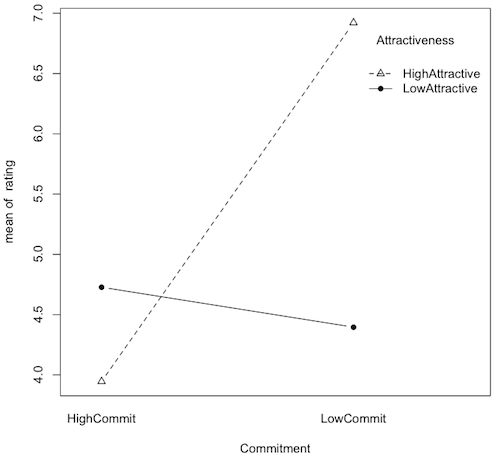
Question 9) What is this graph called (two names)?
Question 10) What effect is most clearly shown on this graph?
> aov.out = aov(rating ~ Commitment * Attractiveness, data=JR89)
> summary(aov.out)
                           Df Sum Sq Mean Sq F value   Pr(>F)
Commitment                  1   87.4   87.42  13.187  0.00036 ***
Attractiveness              1   38.0   38.03   5.737  0.01756 *
Commitment:Attractiveness   1  136.8  136.76  20.630 9.72e-06 ***
Residuals                 196 1299.4    6.63
---
Signif. codes:  0 ‘***’ 0.001 ‘**’ 0.01 ‘*’ 0.05 ‘.’ 0.1 ‘ ’ 1
Prelimary question: Why did that first command line produce no output?
Question 11) Is the main effect of Commitment statistically significant?
Summarize the results of the ANOVA?
Question 12) Is the main effect of Attractiveness statistically significant?
Summarize the results of the ANOVA?
Question 14) Which of these effects is most interesting? Why?
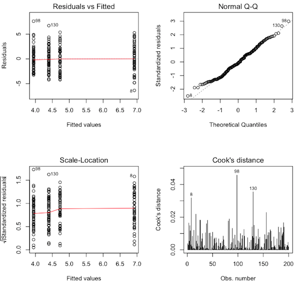
Here's something new! Once you have the aov.out object in your workspace (the result of the ANOVA, whatever you called it), there is an interesting way to check for violations of assumptions graphically. We are going to draw what are called diagnostic plots.
> par(mfrow=c(2,2))  # sets the graphics window for four graphs
> plot(aov.out, 1:4)
Question 15) What are these graphs called? (Hint: you may not know this yet.
Click the check button to find out. You'll be seeing a lot of these in the
future, so read carefully!)
The graph in the upper left corner is called a residuals plot. It is not terribly interesting to us right now. The graph in the upper right corner is called a normal probability plot or a normal Q-Q (quantile-quantile) plot. It is a rough test of the normal distribution assumption. If all of the plotted points on the graph are lined up along the dotted line from lower left to upper right, then normality has been met. Of course, the result is not going to be perfect, because all we have are samples, and samples are what? Noisy! So we can expect some deviations from the dotted line, especially near the ends. What we DON'T want to see are the plotted points forming a pronounced bow (which would indicate skew) or snaking around the dotted line in an S-shaped pattern (to be discussed at a later date). We also don't want to see the plotted points suddenly rising rapidly above the dotted line at the top end or suddenly falling below the dotted line at the lower end (which would indicate outliers).
Question 16) Would you say the normal distribution assumption has been met
by these data? Why?
The graph in the lower left corner is called a scale-location plot. It can be used to check the homogeneity of variance assumption. You'll notice there is a column of plotted points above each of the group means on the horizontal axis. These columns of points should all be roughly the same height. If one of them is dramatically taller or shorter than the others, then homogeneity has been violated. Another way to make the evaluation is to look at the red line. It should be flat. Once again, the result is not going to be perfect because all we have are sample data. We are looking for something reasonably close to what we would expect when variances are homogeneous.
Question 17) Would you say the homogeneity of variance assumption has been met
by these data? Why?
The graph in the lower right corner is called a Cook's distance plot. Cook's distance is calculated for each data point and is plotted as a vertical line on this graph. Cook's distance (or Cook's D) is a measure of how much a data value constitutes an outlier (or "influential point" as we will eventually call it). An outlier is a data value that doesn't seem to go with the rest of the data values in its group, either because it is too large or too small. Such values can have an undue influence on the outcome of the analysis, especially if the groups are small. What we want to see, ideally, in the Cook's distance plot is a freshly mown lawn. (That's a joke!) In other words, we want all the vertical lines to be the same height. Ain't gonna happen. Why not? Because these are sample data, and samples are noisy. So we don't want to see any of the vertical lines being pronouncedly higher than the others. Here, R has flagged three of the data values as potential outliers, cases 8, 98, and 130. Now we have to satisfy ourselves that these data values are not causing a problem, and to do that, we look at the Cook's distances for these points on the vertical axis.
Unfortunately (or fortunately, depending upon how you look at it), there is no universally accepted criterion for what constitutes a large Cook's distance. I can tell you this, however, without fear of being contradicted. A Cook's D of 1.0 or more is definitely a problem. A Cook's D of 0.5 or more is something that needs to be investigated. Here, our Cook's Ds are much tinier than that.
Question 18) Would you say we have any problematic outliers in these data? Why?
It looks like we've passed the assumptions game, so on to something else. We have a significant interaction. To complete our evaluation of this interaction we need to evaluate the simple effects post hoc. (If there was not a signficant interaction but there were significant main effects instead, we would now be considering post hoc tests on the main effects. Here that would be silly. Why? Because each IV contains only two groups, and the ANOVA will tell us whether or not their means are significantly different. We only need post hoc tests on main effects when the interaction is not significant AND the main effect consists of more than two means.) A reminder:
> with(JR89, tapply(rating, list(Attractiveness, Commitment), mean))
               HighCommit LowCommit
HighAttractive   3.945609  6.921761
LowAttractive    4.727338  4.395778
Question 19-22) What are the simple effects?In each case, the simple effect is the effect of one factor at one level of the other. To see an effect of a factor, we have to have at least two means from that factor. So, 3.946 vs. 6.922 is two means from the Commitment factor so it is an effect of Commitment. But they are only the means from one level of Attractiveness, High. So this is a simple effect of Commitment at High Attractiveness. And so on.
How do we test these effects? Right now you should be thinking, "Hey! Two means! Sounds like a t-test to me!" And you'd be right. Because we only have two levels of each factor and, therefore, only two cell means in each simple effect, we can test all the simple effects with Fisher LSD tests. Since there are four tests to be done, we might consider a Bonferroni correction, but I'm going to skip that, and by the time we're done here, you'll know why.
Another reminder. You may remember this from a past slide in the ANOVA lecture.
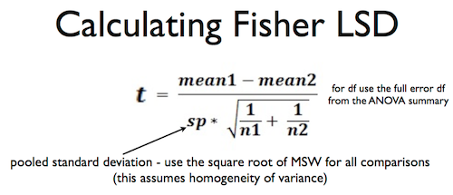
The bottom (denominator) of this formula is the standard error of the mean difference, and it is going to be the same for all four tests because we are assuming homogeneity of variance and all the group sizes are the same. We can get the pooled standard deviation from the ANOVA summary table. How?
But R has shortchanged us on significant figures here. It has only given us three, and it would be good to have more precision than that. Here's how we can get a more precise value for sd.pooled. It is in aov.out.
> aov.out   # no summary() here
Call:
   aov(formula = rating ~ Attractiveness * Commitment, data = JR89)

Terms:
                Attractiveness Commitment Attractiveness:Commitment Residuals
Sum of Squares         38.0303    87.4234                  136.7620 1299.3625
Deg. of Freedom              1          1                         1       196

Residual standard error: 2.574762
Estimated effects may be unbalanced
Remember what I told you once before about residual standard error. Residual standard error is the pooled standard deviation when the data are grouped. Simple as that.
Question 23) What is the value of sd.pooled (do not round)?
Question 24) What is the value of se.meandiff for all four tests (6 decimal
places please)?
Now complete the following table of tests. (Round as little as possible so as to have at least three accurate decimal places in the t-value. Drop any negative signs as these are two-tailed tests. I have calculated the p-values for you in R, as we will see them again below.)
| Tests of Simple Effects | ||||
| Commitment at High Attractiveness |
Commitment at Low Attractiveness |
Attractiveness at High Commitment |
Attractiveness at Low Commitment |
|
| mean difference | ||||
| se.meandiff | ||||
| t-value | ||||
| degrees of freedom | ||||
| p-value | p < .001 | p = 0.520 | p = 0.131 | p < .001 |
This is how you calculate the p-values, just for the hopelessly curious. The first value inside pt() is the t.calc. Always make sure this is positive for a two-tailed test. The second value is df. The option lower.tail=FALSE is a little trick that makes this work. It's multiplied times 2 because this is a two-tailed test.
> pt(5.779475, df=196, lower.tail=F) * 2
[1] 2.911625e-08
> pt(0.6438658, df=196, lower.tail=F) * 2
[1] 0.5204152
> pt(1.5180618, df=196, lower.tail=F) * 2
[1] 0.1306101
> pt(4.9052785, df=196, lower.tail=F) * 2
[1] 1.9555e-06
The problem with testing the simple effects this way is that it's only good for two means. If there are more than two levels of the IV, this test kind of craps out! So here's another way to do it that will work no matter how many means we have to compare. It's going to be an ANOVA (hope you guessed that), but before we do it, I want to reproduce the error line of the ANOVA we've already done. We're going to need it. I'm also going to bump up the precision of these values a bit for the sake of demonstrating something.
             Df   SS      MS
Residuals   196 1299.3625  6.629401
Now we're ready. Watch closely. This is tricky.
> aov.simple1 = aov(rating ~ Commitment, data=JR89, subset=Attractiveness=="HighAttractive")
> print(summary(aov.simple1), digits=8)
            Df    Sum Sq    Mean Sq  F value     Pr(>F)
Commitment   1 221.43705 221.437049 32.00512 1.5247e-07 ***
Residuals   98 678.04252   6.918801
---
Signif. codes:  0 '***' 0.001 '**' 0.01 '*' 0.05 '.' 0.1 ' ' 1
The ANOVA was for rating by Commitment, but only for the subset of ratings that are for High Attractiveness. Therefore, this is (almost) the test of the simple effect of Commitment at High Attractiveness. It is not quite the test, however. Because we are assuming homogeneity of variance, we get to use the error line from the full factorial ANOVA. So the actual test is:
            Df     Sum Sq    Mean Sq  F value
Commitment   1  221.43705 221.437049
Residuals  196 1299.3625    6.629401           ## substituted from overall ANOVA
I've left the F-value blank. You calculate it!
Question 25) What is the F-value for the test of the simple effect of
Commitment at High Attractiveness?
I got a little carried away with decimal places here because I want to demonstrate something. What is the square root of the F-value? It is 5.77947. And where have we seen that value before? I'll wait. Go look for it! Correct! It is the t-value we got from the Fisher LSD test for this same effect. The p-value is also the same (with a little difference in rounding).
> pf(33.402269, df1=1, df2=196, lower.tail=F)
[1] 2.911705e-08
Question 26) Is the simple effect of Commitment at High Attractiveness
statistically significant?
This test is exactly equivalent to the Fisher LSD test when there are only two means. But it also works when there are more than two means.
Now we'll do the rest of them.
> aov.simple2 = aov(rating ~ Commitment, data=JR89, subset=Attractiveness=="LowAttractive")
> print(summary(aov.simple2), digits=8)
            Df    Sum Sq   Mean Sq F value
Commitment   1    2.7483 2.7482985
Residuals  196 1299.3625 6.629401           ## substituted from overall ANOVA
Question 27) What is the F-value for the test of the simple effect of
Commitment at Low Attractiveness?
> pf(0.414562, df1=1, df2=196, lower.tail=F)
[1] 0.5204158
Question 28) Is the simple effect of Commitment at Low Attractiveness
statistically significant?
> aov.simple3 = aov(rating ~ Attractiveness, data=JR89, subset=Commitment=="HighCommit")
> print(summary(aov.simple3), digits=8)
                Df     Sum Sq    Mean Sq F value
Attractiveness   1   15.27751 15.2775082
Residuals      196 1299.3625   6.629401           ## substituted from overall ANOVA

> pf(2.304508, df1=1, df2=196, lower.tail=F)
[1] 0.1306104

> aov.simple4 = aov(rating ~ Attractiveness, data=JR89, subset=Commitment=="LowCommit")
> print(summary(aov.simple4), digits=8)
                Df    Sum Sq   Mean Sq  F value
Attractiveness   1  159.51475 159.51475
Residuals      196 1299.3625    6.629401           ## substituted from overall ANOVA

> pf(24.061713, df1=1, df2=196, lower.tail=F)
[1] 1.95554e-06
Question 29) What is the F-value for the test of the simple effect of
Attractiveness at High Commitment?
Question 30) Is the simple effect of Attractiveness at High Commitment
statistically significant?
Question 31) What is the F-value for the test of the simple effect of
Attractiveness at Low Commitment?
Question 32) Is the simple effect of Attractiveness at Low Commitment
statistically significant?
When all comparisons involve just two means, it's also possible to use the Fisher LSD formula to calculate a least significant difference, or LSD. This is done by finding a t.critical value for the degrees of freedom given and then multiplying that by the se.meandiff (denominator of the t-test formula). In this case, the LSD would be:
> qt(p=0.975, df=196)   # t.critical with 0.025 in the upper tail
[1] 1.972141
> 1.972141 * 0.514952   # t.crit * se.meandiff
[1] 1.015558
Any difference between two means that is larger than this is statistically significant at the alpha=.05 level. If we were worried about inflation of Type I error rates due to the number of comparisons we are doing, we can decrease the alpha level accordingly, which amounts to doing a Bonferroni correction.
> .05 / 4   # Bonferroni corrected alpha for 4 comparisons
[1] 0.0125
> qt(p=0.99375, df=196)   # t.critical with 0.00625 (one-half alpha) in the upper tail
[1] 2.520969
> 2.520969 * 0.514952   # Bonferroni adjusted LSD
[1] 1.298178
Remember how to do this! Someone may ask you. If you don't understand this, ASK, ASK, ASK!
We have not calculated effect sizes yet. We will use eta-squared as our effect size statistic. For that, we will need to get SS.total.
Question 33) What is SS.total?
Questions 34-36) What are the following eta-squared values?
Commitment: eta-sq =
Attractiveness: eta-sq =
Commitment-by-Attractiveness: eta-sq =
Question 37) How would you evaluate the size of these effects?
Question 38) Well in that case, how is it that some of these effects have such
small p-values?
Question 39) The hypothesis that people in commited relationships devalue
attractive or threatening alternative partners is:
Question 40) Did the researchers find evidence that people in commited
relationships devalue potential alternative partners even if they are not
attractive?
Question 41) Both main effects were statistically significant. How would the
main effect of Commitment be described?
Question 42) Was what you said in question 41 true for both high attractive
and low attractive alternative partners?
The End