That sounds complicated enough, doesn't it? It's not. As you already know, it's just another thing we can do with multiple regression. When a multiple regression analysis includes both numeric and categorical predictors, it's called analysis of covariance or ANCOVA. Some people prefer to reserve the name ANCOVA to a more restricted range of problems, but we'll get to that.
Here's the graph from the article you just read. I enlarged it a little and put some grid lines on it, the reason being that I wanted to extract the data from it. This is today's problem.
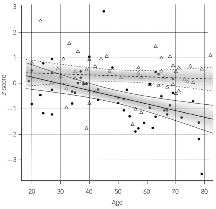
It looks like a scatterplot with two regression lines on it, and that's exactly what it is. The response on the vertical axis is volume of the hippocampus, which has been standardized (an unnecessary step, but convenient as it allows us to easily visual effect sizes--remember Cohen's d). On the horizontal axis we have age, also a numeric variable. The third variable in this regression is categorical. I've called it "diagnosis" in the dataset at the website, and there are two levels of that: normal controls and patients diagnosed as schizophrenic. The points from the normal controls are the white triangles, and the black circles are the patients. There is a regression line for each of those groups. This is an ANCOVA. (The gray shaded areas are confidence intervals around the regression lines, an unnecessary but very classy touch. It's possible to do that in R, but I can never remember how.)
Try to ignore the regression lines for a moment and just look at the points. Would it have been obvious to you that there are different effects of age for the normal controls (triangles) and schizophrenic patients (black balls)? They appear to be fairly well mixed together, don't they? The difference becomes fairly obvious near the right edge of the graph, where the triangles tend to be higher than the black balls. On the left edge of the graph, they are pretty well mixed.
You can see in this scatterplot (and you also read it in the article) that the two predictors are interacting. The two regression lines are not parallel. Hippocampal size decreases only slightly with age in the normal control subjects but decreases more dramatically in the schizophrenic patients. I have extracted the data from this graph as best I could and have put it into a data file called hippocampus2.txt at the website.
Before we get to that though, I have also created another dataset, called hippocampus1.txt, which is also at the website. In that dataset I have artificially removed the age-by-diagnosis interaction by flattening (reducing the slope of) the line for the schizophrenic patients. It's easier to understand ANCOVA if you don't have to deal with an interaction, so we'll look at that dataset first. (Thus, this will be the answer to one of the practice problems from the ANCOVA lecture.)
> rm(list=ls())
> file = "http://ww2.coastal.edu/kingw/psyc480/data/hippocampus1.txt"
> hippo1 = read.table(file=file, header=T, stringsAsFactors=T)
> summary(hippo1)
     volume             age         diagnosis
 Min.   :-2.8000   Min.   :19.00   normal:49
 1st Qu.:-0.8000   1st Qu.:36.00   schizo:50
 Median :-0.1000   Median :52.00
 Mean   :-0.1121   Mean   :50.81
 3rd Qu.: 0.6000   3rd Qu.:66.00
 Max.   : 2.7000   Max.   :82.00
As you can see in the summary, we have a volume variable that has been converted to z-scores representing the volume of the hippocampus, a structure in the temporal lobe of the brain that has to do with memory and spatial cognition, we have an age variable, which is age in years, and we have a diagnosis variable.
The point of ANCOVA is often to see the effect of a categorical variable with some numeric variable, perhaps a confounder, removed. This numeric variable, which is there only for control purposes, is called a "numeric covariate," the idea being that it is related to the categorical IV we are really interested in and, therefore, we want variability due to the covariate removed before we test the categorical IV of interest. In this case, the numeric variable is age. We want to see the effect of diagnosis on hippocampal size after age has been removed. The hippocampus tends to shrink a bit with age, so controlling for (or removing) the effect of age might make the effect of diagnosis clearer.
The analysis can be done either by ANOVA or by regression. I'll show you how to do it by ANOVA later. I think regression is the more sensible way to do it in this case. Let's get some means first.
> with(hippo1, tapply(volume, diagnosis, mean))
    normal     schizo
 0.2836735 -0.5000000
As you can see, the hippocampus in the normal brain is larger by about three-quarters of a standard deviation. In fact, keep in mind that the difference between these means is 0.28 - (-0.50) = 0.78 SDs. These means have not taken into account the effect of age or, as they say in ANCOVA, these means are not adjusted for age.
Age would be a confound in this analysis if one group were older than the other. If the schizophrenic patients are older on the average, then we might expect them to have smaller hippocampi because the hippocampus shrinks with age. In this case, there isn't much difference in the age of the two groups, so adjusting the means for age won't have much of an effect. But it will have a little because, as it turns out, the control subjects are older, on the average, by a little more than 3 years. (You can check that for yourself if you're curious.)
> lm.hippo1 = lm(volume ~ age * diagnosis, data=hippo1)
> summary(lm.hippo1)

Call:
lm(formula = volume ~ age * diagnosis, data = hippo1)

Residuals:
    Min      1Q  Median      3Q     Max
-2.1437 -0.4311 -0.0381  0.4775  3.1782

Coefficients:
                     Estimate Std. Error t value Pr(>|t|)
(Intercept)          0.460795   0.401629   1.147    0.254
age                 -0.003374   0.007280  -0.464    0.644
diagnosisschizo     -0.703224   0.541549  -1.299    0.197
age:diagnosisschizo -0.001865   0.010070  -0.185    0.853

Residual standard error: 0.8656 on 95 degrees of freedom
Multiple R-squared:  0.1815,	Adjusted R-squared:  0.1557
F-statistic: 7.022 on 3 and 95 DF,  p-value: 0.0002576
In this analysis, age has been entered as a "numeric covariate." I have entered it first because I'm superstitious. In a standard multiple regression, it doesn't matter since each predictor is treated as if entered last. I'm also checking for an interaction by using * instead of +. There is none, p = 0.853, so I'm going to redo the analysis and drop the interaction term. In regression analysis, nonexistent interactions should be dropped and the regression redone without them. (Why isn't that true in ANOVA? Beats me!)
> lm.hippo1 = lm(volume ~ age + diagnosis, data=hippo1)
> summary(lm.hippo1)

Call:
lm(formula = volume ~ age + diagnosis, data = hippo1)

Residuals:
    Min      1Q  Median      3Q     Max
-2.1702 -0.4302 -0.0249  0.4785  3.1819

Coefficients:
                 Estimate Std. Error t value Pr(>|t|)
(Intercept)      0.511959   0.290067   1.765   0.0807 .
age             -0.004349   0.005004  -0.869   0.3870
diagnosisschizo -0.798155   0.173925  -4.589 1.35e-05 ***
---
Signif. codes:  0 '***' 0.001 '**' 0.01 '*' 0.05 '.' 0.1 ' ' 1

Residual standard error: 0.8612 on 96 degrees of freedom
Multiple R-squared:  0.1812,	Adjusted R-squared:  0.1641
F-statistic: 10.62 on 2 and 96 DF,  p-value: 6.798e-05
Now we see what we're looking for--the effect of diagnosis after the effect of age has been removed. That is given in the third line of the coefficients, which is labeled "diagnosisschizo," which means this is the effect of being diagnosed with schizophrenia (as compared to the normal controls). The coefficient, -0.798155, call it -0.80, is the difference in the adjusted means, or the difference in the means after they have been adjusted for age. Notice also that this difference is statistically significant, t(96) = -4.589, p < .001. So the result is that being a member of the group diagnosed with schizophrenia reduces (negative coefficient) your hippocampal size by 0.80 SDs (the hippocampal sizes have been standardized, so the units of measurement here are SDs).
Can the means adjusted for age be calculated? Yes, they can, and I'll show you how, but it's my opinion that the difference in the adjusted means and the test on that difference, as given in the regression result, is the important finding. To calculate the adjusted means:
Compare these to the unadjusted means calculated above. The adjusted means haven't changed much (I said they wouldn't), but they have changed a little.
Drawing the scatterplot would be tricky and would involve a more sophisticated knowledge of R, and I'm not going to explain it (unless you ask me specifically), but these are the commands that would be used for those of you who want to fool with it. (You can draw anything you want in an R graphics window. I once said I could draw a clown face in an R graphics window if I wanted to. In fact, I said it for years with no reaction from the students, until one semester, the students challenged me to do it. So I did.)
**********You do not need to know how to do this. Ask it curious.**********
> plot(volume ~ age, data=hippo1, ylim=c(-3,3), col="white")
> points(hippo1$age[hippo1$diagnosis=="normal"], hippo1$volume[hippo1$diagnosis=="normal"], pch=2)
> abline(a=0.5120, b=-0.004349, lty="dashed")
> points(hippo1$age[hippo1$diagnosis=="schizo"], hippo1$volume[hippo1$diagnosis=="schizo"], pch=19)
> abline(a=0.5120-.7982, b=-0.004349, lty="solid")
***************************************************************************
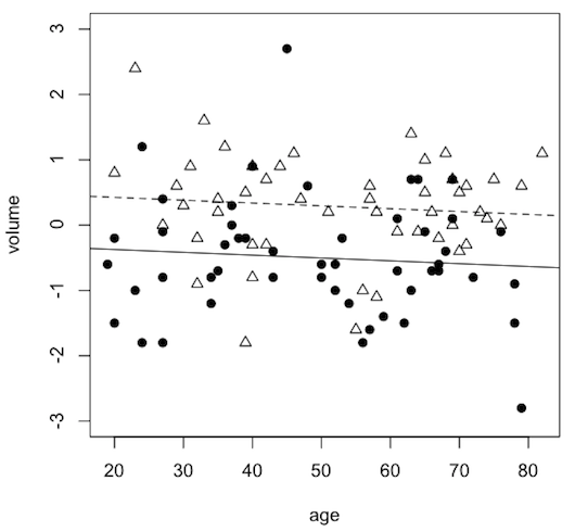
What the points and lines represent would then have to be explained in a legend or a caption, but they are the same as they were in the researcher's graph.
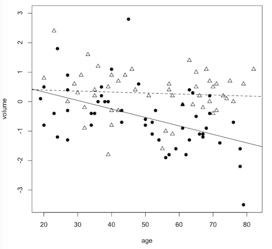
We will now move on to the "real" data, in which the researchers found an interaction.
> rm(list=ls())   # clear your workspace
> file = "http://ww2.coastal.edu/kingw/psyc480/data/hippocampus2.txt"
> hippo2 = read.table(file=file, header=T, stringsAsFactors=T)
> summary(hippo2)
     volume             age         diagnosis
 Min.   :-3.5000   Min.   :19.00   normal:49
 1st Qu.:-0.8000   1st Qu.:36.00   schizo:50
 Median : 0.0000   Median :52.00
 Mean   :-0.1182   Mean   :50.81
 3rd Qu.: 0.5000   3rd Qu.:66.00
 Max.   : 2.8000   Max.   :82.00
The variables have already been explained, so without any further time-wasting blather, let's get straight to the regression analysis.
> lm.hippo2 = lm(volume ~ age * diagnosis, data=hippo2)
> summary(lm.hippo2)

Call:
lm(formula = volume ~ age * diagnosis, data = hippo2)

Residuals:
    Min      1Q  Median      3Q     Max
-2.1292 -0.4305 -0.0469  0.4702  3.1922

Coefficients:
                     Estimate Std. Error t value Pr(>|t|)
(Intercept)          0.460795   0.400080   1.152   0.2523
age                 -0.003374   0.007252  -0.465   0.6428
diagnosisschizo      0.443384   0.539462   0.822   0.4132
age:diagnosisschizo -0.025433   0.010031  -2.535   0.0129 *
---
Signif. codes:  0 '***' 0.001 '**' 0.01 '*' 0.05 '.' 0.1 ' ' 1

Residual standard error: 0.8623 on 95 degrees of freedom
Multiple R-squared:  0.2887,	Adjusted R-squared:  0.2663
F-statistic: 12.86 on 3 and 95 DF,  p-value: 4.041e-07
I must have done a reasonably good job of copying the data off the figure in the article because I got very nearly the same result. The interaction is significant, p = 0.0129 (the authors got p = 0.012). The authors used an F-test to test the significance of the interaction coefficient, but F = t2, so our F-test is F(1,95) = 2.535^2 = 6.43 (the authors got 6.57).
Many people consider the point of ANCOVA to be simply the removal of an effect of a confounding numeric covariate, or to reduce variability in the response by removing the effect of a covariate, and in that case we wouldn't want an interaction. An interaction would toss a monkey wrench into those works. In fact, in some textbooks, you will read that an assumption of ANCOVA is that there is no interaction. However, in the broader sense in which we are using ANCOVA (some predictors numeric, some categorical), interactions are fine. As always, when they exist, they are the most interesting effect.
In this study, the whole point was to find the interaction. We know that the hippocampus degenerates (slightly!) with age. We also know that schizophrenia is accompanied by a degeneration in the hippocampus. Combine age with schizophrenia and it is entirely reasonable to hypothesize that the hippocampus in schizophrenia would lose volume more rapidly with age than it would in normal controls. In other words, the slope of the schizophrenia line should be steeper on the scatterplot than the slope of the normal control line. That's an interaction.
What would those slopes be? Let's write the regression equation.
volume.hat = 0.4608 - 0.003374 * age + 0.4434 * diagnosisschizo - 0.025433 * age * diagnosisschizo
The way the diagnosis term is coded in the regression table tells us that diagnosisschizo=1 for the schizophrenic patients and 0 for the normal controls. Hence:
volume.hat = 0.4608 - 0.003374 * age + 0.443384 * 0 - 0.025433 * age * 0
           = 0.4608 - 0.003374 * age (for normal control subjects)
volume.hat = 0.4608 - 0.003374 * age + 0.443384 * 1 - 0.025433 * age * 1
           = 0.9042 - 0.028807 * age  (for schizophrenic patients)
The slope for the normal control subjects is -0.003374 and for the schizophrenic patients is -0.028807, which is a steeper line. Can you interpret them? The units of age is years, so the volume of a normal person's hippocampus is predicted to decline by 0.003374 SDs per year, on the average, while the hippocampus of schizophrenic patients is predicted to decline by 0.028807 SDs per year, on the average.
ASIDE: In cases such as we have here, where there is one numeric variable and one two-level categorical variable, there is an easier way to get those slopes. Do you see it? Hint: remember what the definition of an interaction is. Here is the Answer.
Is that difference in slopes statistically significant? Well, yeah, that's what the test on the interaction term in the regression is telling us. Here we're not interested so much in the difference between the means. If there is no interaction, then the difference in the means is predicted to be the same at all ages, but with the interaction the difference in the group means changes with age. With the interaction we are interested in the difference in the slopes.
For people who have to know, here's how you would draw the scatterplot.
**********You do not need to know how to do this. Ask it curious.**********
> plot(volume ~ age, data=hippo2, ylim=c(-3.5,3), col="white")
> points(hippo2$age[hippo2$diagnosis=="normal"], hippo2$volume[hippo2$diagnosis=="normal"], pch=2)
> abline(a=0.4608, b=-0.003374, lty="dashed")
> points(hippo2$age[hippo2$diagnosis=="schizo"], hippo2$volume[hippo2$diagnosis=="schizo"], pch=19)
> abline(a=0.9042, b=-0.02881, lty="solid")
***************************************************************************
Can we do this as an ANOVA? No problem!
> summary(aov(volume ~ age * diagnosis, data=hippo2))
              Df Sum Sq Mean Sq F value   Pr(>F)
age            1   6.13   6.130   8.244  0.00504 **
diagnosis      1  17.76  17.765  23.893 4.13e-06 ***
age:diagnosis  1   4.78   4.780   6.428  0.01286 *
Residuals     95  70.63   0.744
---
Signif. codes:  0 '***' 0.001 '**' 0.01 '*' 0.05 '.' 0.1 ' ' 1

                    SS       delta R-squared      p-value
age               6.13    6.13 / 99.30 = 0.0617   0.00504
diagnosis        17.76   17.76 / 99.30 = 0.1789   < .001
age x diagnosis   4.78    4.78 / 99.30 = 0.0481   0.01286
residuals        70.63
                ------
SS.total         99.30
What if there are more than two levels of the categorical variable? It's basically the same procedure.
> rm(list=ls())
> data(anorexia, package="MASS")
> summary(anorexia)
  Treat        Prewt           Postwt
 CBT :29   Min.   :70.00   Min.   : 71.30
 Cont:26   1st Qu.:79.60   1st Qu.: 79.33
 FT  :17   Median :82.30   Median : 84.05
           Mean   :82.41   Mean   : 85.17
           3rd Qu.:86.00   3rd Qu.: 91.55
           Max.   :94.90   Max.   :103.60
These are data supposedly from a study on the treatment of anorexia in women, although I've never seen it published anywhere and, frankly, I'm a little skeptical of the results. Nevertheless, it is a classic example of ANCOVA. (There are two other ways these data might be analyzed. How? Answer: mixed factorial ANOVA, and single-factor between groups ANOVA on the diffs=Postwt-Prewt scores.)
> head(anorexia)
  Treat Prewt Postwt
1  Cont  80.7   80.2
2  Cont  89.4   80.1
3  Cont  91.8   86.4
4  Cont  74.0   86.3
5  Cont  78.1   76.1
6  Cont  88.3   78.1
Each line of the data frame is one subject, so it is a wide format data frame. There are three variables:
When I do this analysis, I want to be sure R sees "Cont" as the baseline or control group to which the other two groups will be compared, so I am going to make sure R sees it that way right now!
> anorexia$Treat = relevel(anorexia$Treat, ref="Cont")
If that syntax looks a little tortured, well, it is. The relevel function creates the base or reference level of the factor, but then the factor has to be assigned back to itself. Otherwise, the releveling won't stick. Remember: if we are going to create or change something in the workspace, an equals sign (=), is going to be involved somehow. We can make sure it is sticking as follows.
> levels(anorexia$Treat)
[1] "Cont" "CBT"  "FT"
The first level listed is the reference level, the group to which all other groups will be compared. Ordinarily, R would just put the levels in alphabetical order and, thereby, treat "CBT" as the reference level. We just told it not to do that. It's always nice to have your control group be the reference level.
Note: This variable cannot be dummy coded. Why not? Answer: weeeellllll, actually it can, but it's complicated. What you cannot do, however, is code those levels 0/1/2 or 1/2/3 and then enter those numbers into a regression analysis. That is meaningless. It would also be meaningless to calculate correlations with such codes.
Now let's get some means.
> with(anorexia, tapply(Prewt, Treat, mean))
    Cont      CBT       FT
81.55769 82.68966 83.22941
> with(anorexia, tapply(Postwt, Treat, mean))
    Cont      CBT       FT
81.10769 85.69655 90.49412
Does that look like an interaction to you? Yeah, me too. We're going to ignore that for the time being. (But why should we have expected it?)
Notice that the FT (family therapy) subjects weighed the most, on average, after the treatment, but they also weighed the most before treatment. We want that pretreatment weight bias removed before we look at posttreatment weights. This sounds like a job for ANCOVA. Treat will be the IV we are interested in and Prewt will be entered as a numeric covariate.
> lm.anorexia =lm(Postwt ~ Prewt + Treat, data=anorexia)
> summary(lm.anorexia)

Call:
lm(formula = Postwt ~ Prewt + Treat, data = anorexia)

Residuals:
     Min       1Q   Median       3Q      Max
-14.1083  -4.2773  -0.5484   5.4838  15.2922

Coefficients:
            Estimate Std. Error t value Pr(>|t|)
(Intercept)  45.6740    13.2167   3.456 0.000950 ***
Prewt         0.4345     0.1612   2.695 0.008850 **
TreatCBT      4.0971     1.8935   2.164 0.033999 *
TreatFT       8.6601     2.1931   3.949 0.000189 ***
---
Signif. codes:  0 '***' 0.001 '**' 0.01 '*' 0.05 '.' 0.1 ' ' 1

Residual standard error: 6.978 on 68 degrees of freedom
Multiple R-squared:  0.2777,	Adjusted R-squared:  0.2458
F-statistic: 8.713 on 3 and 68 DF,  p-value: 5.719e-05
Now we can write a regression equation.
Postwt.hat = 45.6740 + 0.4345 * Prewt + 4.0971 * TreatCBT + 8.6601 * TreatFT
Again looking at the coefficients, the model is telling us that the difference between the adjusted means for "Cont" (the reference level) and "CBT" was 4.0971 pounds, CBT higher since the coefficient for TreatCBT is positive (that is the effect of TreatCBT), and that difference is statistically significant, p = 0.034. The difference between the adjusted means for "Cont" and "FT" was 8.6601 pounds, in favor of FT, and that difference is also statistically significant, p < .001. The difference between the adjusted means for "CBT" and "FT" was 8.6601 - 4.0971 = 4.5630 pounds, but there is no test on that difference.
The adjusted means can be calculated in the usual way by substituting the overall preweight mean for Prewt. Put 1 (one) in for the group you're calculating the mean for, and zero for everybody else.
Postwt.hat = 45.6740 + 0.4345 * Prewt + 4.0971 * TreatCBT + 8.6601 * TreatFT
           = 45.6740 + 0.4345 * 82.41 + 4.0971 * 0 + 8.6601 * 0
           = 81.4811 (for Cont)
           = 45.6740 + 0.4345 * 82.41 + 4.0971 * 1 + 8.6601 * 0
           = 85.5782 (for CBT)
           = 45.6740 + 0.4345 * 82.41 + 4.0971 * 0 + 8.6601 * 1
           = 90.1412 (for FT)
The ANCOVA can also be done by ANOVA, and once again I'll leave out the interaction term to avoid confusing ourselves.
> aov.anorexia = aov(Postwt ~ Prewt + Treat, data=anorexia)
> summary(aov.anorexia)
            Df Sum Sq Mean Sq F value   Pr(>F)
Prewt        1    507   506.5  10.402 0.001936 **
Treat        2    766   383.1   7.868 0.000844 ***
Residuals   68   3311    48.7
---
Signif. codes:  0 '***' 0.001 '**' 0.01 '*' 0.05 '.' 0.1 ' ' 1
In this case, the numeric covariate MUST be entered first because, remember, these are Type I or sequential sums of squares, and we want Prewt out before Treat is tested. I think we get a lot less information this way, but we do get one new thing.
SS.total = 507 + 766 + 3311 = 4584
delta.R-squared.Treat = 766 / 4584 = 0.1671
Quite a lot of the explained variability is actually due to the covariate. Treat accounts for 16.71% of the total variability in Postwt.
We could have gotten the delta R-squareds using lm(), too. Can you figure out how? Hint: we would have to use it twice.
**********You do not need to know how to do this. Ask it curious.**********
Now I'm going to show you how to dummy code a categorical variable that has more than two levels. If you don't what to know this, don't watch. This is just for the hopelessly curious.
> anorexia   # I have deleted some lines from the output to save space
   Treat Prewt Postwt
1   Cont  80.7   80.2
2   Cont  89.4   80.1
3   Cont  91.8   86.4
...
24  Cont  77.5   81.2
25  Cont  72.3   88.2
26  Cont  89.0   78.8
27   CBT  80.5   82.2
28   CBT  84.9   85.6
29   CBT  81.5   81.4
...
53   CBT  84.5   84.6
54   CBT  80.8   96.2
55   CBT  87.4   86.7
56    FT  83.8   95.2
57    FT  83.3   94.3
58    FT  86.0   91.5
...
70    FT  89.9   93.8
71    FT  86.0   91.7
72    FT  87.3   98.0
We want to dummy code Treat. There is nothing to stop us from coding it 1/2/3, but those would NOT be dummy codes, and they could NOT be used in statistical analyses unless declared as a factor. Dummy codes (as far as we're concerned) are 0/1 and that's it. How could we code a three level factor using just 0/1?
The answer is, we have to create more than one dummy coded variable. Generally, we will need one less dummy coded variable than our factor has levels. I'm going to create two dummy coded variables. One will be called CBT and will be coded as 1 for subjects who are members of that group and 0 otherwise. The other will be called FT, and will be coded as 1 for subjects who are members of that group and 0 otherwise. What about the controls? Think about it. If you're 0 on CBT and 0 on FT, then you're in the control group. We don't need separate dummy codes for the baseline or reference group.
Watch carefully. I'm about to be very clever, and I wouldn't want you to miss it!
> anorexia$CBT = ifelse(anorexia$Treat=="CBT", yes=1, no=0)
> anorexia$FT = ifelse(anorexia$Treat=="FT", yes=1, no=0)
> anorexia   # some lines of output omitted
   Treat Prewt Postwt CBT FT
1   Cont  80.7   80.2   0  0
2   Cont  89.4   80.1   0  0
3   Cont  91.8   86.4   0  0
...
24  Cont  77.5   81.2   0  0
25  Cont  72.3   88.2   0  0
26  Cont  89.0   78.8   0  0
27   CBT  80.5   82.2   1  0
28   CBT  84.9   85.6   1  0
29   CBT  81.5   81.4   1  0
...
53   CBT  84.5   84.6   1  0
54   CBT  80.8   96.2   1  0
55   CBT  87.4   86.7   1  0
56    FT  83.8   95.2   0  1
57    FT  83.3   94.3   0  1
58    FT  86.0   91.5   0  1
...
70    FT  89.9   93.8   0  1
71    FT  86.0   91.7   0  1
72    FT  87.3   98.0   0  1
Now we do the regression with the covariate and the two dummy coded variables.
> lm.anorexia2 = lm(Postwt ~ Prewt + CBT + FT, data=anorexia)
> summary(lm.anorexia2)

Call:
lm(formula = Postwt ~ Prewt + CBT + FT, data = anorexia)

Residuals:
     Min       1Q   Median       3Q      Max
-14.1083  -4.2773  -0.5484   5.4838  15.2922

Coefficients:
            Estimate Std. Error t value Pr(>|t|)
(Intercept)  45.6740    13.2167   3.456 0.000950 ***
Prewt         0.4345     0.1612   2.695 0.008850 **
CBT           4.0971     1.8935   2.164 0.033999 *
FT            8.6601     2.1931   3.949 0.000189 ***
---
Signif. codes:  0 ‘***’ 0.001 ‘**’ 0.01 ‘*’ 0.05 ‘.’ 0.1 ‘ ’ 1

Residual standard error: 6.978 on 68 degrees of freedom
Multiple R-squared:  0.2777,	Adjusted R-squared:  0.2458
F-statistic: 8.713 on 3 and 68 DF,  p-value: 5.719e-05
Compare this result to summary(lm.anorexia) above.
***************************************************************************